ISAAC
This is a plugin for the in-situ library ISAAC [Matthes2016] for a live rendering and steering of PIConGPU simulations.
External Dependencies
The plugin is available as soon as the ISAAC library is compiled in.
.cfg file
Command line option |
Description |
|---|---|
|
Sets up, that every N th timestep an image will be rendered. This parameter can be changed later with the controlling client. |
|
Sets the NAME of the simulation, which is shown at the client. |
|
URL of the required and running isaac server. Host names and IPs are supported. |
|
PORT of the isaac server.
The default value is |
|
Setups the WIDTH and HEIGHT of the created image(s). |
|
Default is |
|
If activated (argument set to |
|
Sets the QUALITY of the images, which are compressed right after creation.
Values between |
|
Enable and write benchmark results into the given file. |
The most important settings for ISAAC are --isaac.period, --isaac.name and --isaac.url.
A possible addition for your submission tbg file could be --isaac.period 1 --isaac.name !TBG_jobName --isaac.url YOUR_SERVER, where the tbg variables !TBG_jobName is used as name and YOUR_SERVER needs to be set up by yourself.
.param file
The ISAAC Plugin has an isaac.param, which specifies which fields and particles are rendered. This can be edited (in your local paramSet), but at runtime also an arbitrary amount of fields (in ISAAC called sources) can be deactivated. At default every field and every known species are rendered.
Running and steering a simulation
First of all you need to build and run the isaac server somewhere. On HPC systems, simply start the server on the login or head node since it can be reached by all compute nodes (on which the PIConGPU clients will be running).
Functor Chains
One of the most important features of ISAAC are the Functor Chains.
As most sources (including fields and species) may not be suited for a direct rendering or even full negative (like the electron density field), the functor chains enable you to change the domain of your field source-wise. A date will be read from the field, the functor chain applied and then only the x-component used for the classification and later rendering of the scene.
Multiply functors can be applied successive with the Pipe symbol |.
The possible functors are at default:
mul for a multiplication with a constant value. For vector fields you can choose different value per component, e.g.
mul(1,2,0), which will multiply the x-component with 1, the y-component with 2 and the z-component with 0. If less parameters are given than components exists, the last parameter will be used for all components without an own parameter.add for adding a constant value, which works the same as
mul(...).sum for summarizing all available components. Unlike
mul(...)andadd(...)this decreases the dimension of the data to1, which is a scalar field. You can exploit this functor to use a different component than the x-component for the classification, e.g. withmul(0,1,0) | sum. This will first multiply the x- and z-component with 0, but keep the y-component and then merge this to the x-component.length for calculating the length of a vector field. Like sum this functor reduces the dimension to a scalar field, too. However
mul(0,1,0) | sumandmul(0,1,0) | lengthdo not do the same. Aslengthdoes not know, that the x- and z-component are 0 an expensive square root operation is performed, which is slower than just adding the components up.idem does nothing, it just returns the input data. This is the default functor chain.
Beside the functor chains the client allows to setup the weights per source (values greater than 6 are more useful for PIConGPU than the default weights of 1), the classification via transfer functions, clipping, camera steering and to switch the render mode to iso surface rendering. Furthermore interpolation can be activated. However this is quite slow and most of the time not needed for non-iso-surface rendering.
Memory Complexity
Accelerator
locally, a framebuffer with full resolution and 4 byte per pixel is allocated.
For each FieldTmp derived field and FieldJ a copy is allocated, depending on the input in the isaac.param file.
Host
negligible.
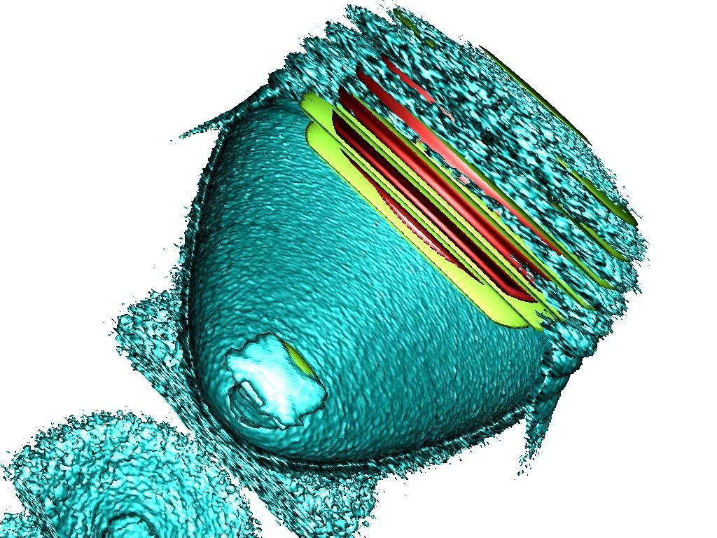
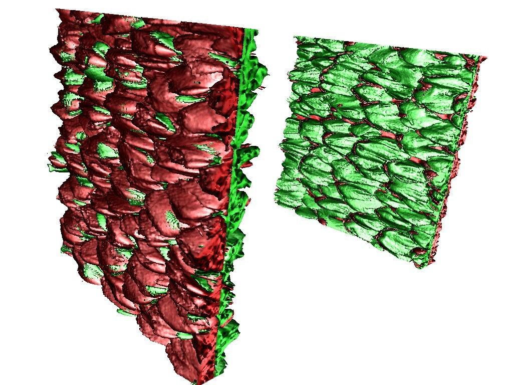
Example renderings

References
A. Matthes, A. Huebl, R. Widera, S. Grottel, S. Gumhold, and M. Bussmann In situ, steerable, hardware-independent and data-structure agnostic visualization with ISAAC, Supercomputing Frontiers and Innovations 3.4, pp. 30-48, (2016), arXiv:1611.09048, DOI:10.14529/jsfi160403