Finite-Difference Time-Domain Method
Section author: Klaus Steiniger, Jakob Trojok, Sergei Bastrakov
For the discretization of Maxwell’s equations on a mesh in PIConGPU, only the equations
are solved. This becomes possible, first, by correctly solving Gauss’s law \(\nabla \cdot \vec{E} = \frac{1}{\varepsilon_0}\sum_s \rho_s\) using Esirkepov’s current deposition method [Esirkepov2001] (or variants thereof) which solve the discretized continuity equation exactly. Second, by assuming that the initially given electric and magnetic field satisfy Gauss’ laws. Starting simulations in an initially charge free and magnetic-divergence-free space, i.e.
is standard in PIConGPU. Alternatively, one could use non-charge-free initialization and solve the Poisson equation for initial values of \(\vec{E}\).
Discretization on a staggered mesh
In the Finite-Difference Time-Domain method, above Maxwell’s equations are discretized by replacing the partial space and time derivatives with centered finite differences. For example, the partial space derivative along \(x\) of a scalar field \(u\) at position \((i,j,k)\) and time step \(n\) becomes
and the temporal derivative becomes
when replacing with the lowest order central differences. Note, with this leapfrog discretization or staggering, derivatives of field quantities are calculated at positions between positions where the field quantities are known.
The above discretization uses one neighbor to each side from the point where the derivative is calculated yielding a second order accurate approximation of the derivative. Using more neighbors for finite difference calculation of the spatial derivatives is possible in PIConGPU and increases the approximation order of these derivatives. Note, however, that the order of the whole Maxwell’s solver also depends on accuracy of \(\vec{J}\) calculation on the grid. For those values PIConGPU provides only second-order accuracy in terms of time and spatial grid steps (as the underlying discretized continuity equation is of that order) regardless of the chosen field solver. Thus, in the general case the Maxwell’s solver as a whole still has second order accuracy in space, and only provides arbitrary order in finite difference approximation of curls.
For the latter, the accuracy order scales with twice the number of neighbors \(M\) used to approximate the derivative. The arbitrary order finite difference derivative approximation of order \(2M\) reads
with \(l=-M+1/2, -M+1+1/2, ..., -1/2, 1/2, ..., M-1/2\) [Ghrist2000]. A recurrence relation for the weights exists,
Maxwell’s equations on the mesh
When discretizing on the mesh with centered finite differences, the spatial positions of field components need to be chosen such that a field component, whose temporal derivative is calculated on the left hand side of a Maxwell equation, is spatially positioned between the two field components whose spatial derivative is evaluated on the right hand side of the respective Maxwell equation. In this way, the spatial points where a left hand side temporal derivative of a field is evaluated lies exactly at the position where the spatial derivative of the right hand side fields is calculated. The following image visualizes the arrangement of field components in PIConGPU.

Component-wise and using second order finite differences for the derivative approximation, Maxwell’s equations read in PIConGPU
As can be seen from these equations, the components of the source current are located at the respective components of the electric field. Following Gauss’s law, the charge density is located at the cell corner.
Using Esirkepov’s notation for the discretized differential operators,
the shorthand notation for the discretized Maxwell equations in PIConGPU reads
with initial conditions
The components \(E_x\rvert_{1/2, 0, 0}=E_y\rvert_{0, 1/2, 0}=E_z\rvert_{0, 0, 1/2} =B_x\rvert_{I, J+1/2, K+1/2}=B_y\rvert_{I+1/2, J, K+1/2}=B_z\rvert_{I+1/2, J+1/2, K}=0\) for all times when using absorbing boundary conditions. Here, \(I,J,K\) are the maximum values of \(i,j,k\) defining the total mesh size.
Note, in PIConGPU the \(\vec B\)-field update is split in two updates of half the time step, e.g.
and
for the \(B_x\) component, where the second half of the update is performed at the beginning of the next time step such that the electric and magnetic field are known at equal time in the particle pusher and at the end of a time step.
Dispersion relation of light waves on a mesh
The dispersion relation of a wave relates its oscillation period in time \(T\) to its oscillation wavelength \(\lambda\), i.e. its angular frequency \(\omega = \frac{2\pi}{T}\) to wave vector \(\vec k = \frac{2\pi}{\lambda} \vec e_k\). For an electromagnetic wave in vacuum,
However, on a 3D mesh, with arbitrary order finite differences for the spatial derivatives, the dispersion relation becomes
where \(\tilde k_x\), \(\tilde k_y\), and \(\tilde k_z\) are the wave vector components on the mesh in \(x\), \(y\), and \(z\) direction, respectively. As is obvious from the relation, the numerical wave vector will be different from the real world wave vector for a given frequency \(\omega\) due to discretization.
Dispersion Relation for Yee’s Method
Yee’s method [Yee1966] uses second order finite differences for the approximation of spatial derivatives. The corresponding dispersion relation reads
Obviously, this is a special case of the general dispersion relation, where \(M=1\).
Solving for a wave’s numerical frequency \(\omega\) in dependence on its numerical wave vector \(\vec{\tilde k} = (\tilde k\cos\phi\sin\theta, \tilde k\sin\phi\sin\theta, \tilde k\cos\theta)\) (spherical coordinates),
where
Denoting
we have \(\xi \leq \xi_\mathrm{max}\) with equality possible for diagonal wave propagation and a certain relation between time and spatial grid steps.
This reveals two important properties of the field solver. (The 2D version is obtained by letting \(\tilde k_z = 0\).)
First, only within the range \(\xi_\mathrm{max} \leq 1\) the field solver operates stably. This gives the Courant-Friedrichs-Lewy stability condition relating time step to mesh spacing
Typically, \(\xi_\mathrm{max} = 0.995\) is chosen. Outside this stability region, the frequency \(\omega\) corresponding to a certain wave vector becomes imaginary, meaning that wave amplitudes can be nonphysically exponentially amplified [Taflove2005].
Second, there exists a purely numerical anisotropy in a wave’s phase velocity \(\tilde v_p = \omega / \tilde k\) (speed of electromagnetic wave propagation) depending on its propagation direction \(\phi\), as depicted in the following figure
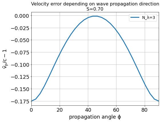
assuming square cells \(\Delta x = \Delta y = \Delta\) and where \(S=c\Delta t / \Delta\), \(N_\lambda=\lambda/\Delta\). That is, for the chosen sampling of three samples per wavelength \(\lambda\), the phase velocities along a cell edge and a cell diagonal differ by approximately 20%. The velocity error is largest for propagation along the edge. The phase velocity error can be significantly reduced by increasing the sampling, as visualized in the following figure by the scaling of the velocity error with wavelength sampling for propagation along the cell edge

Another conclusion from this figure is, that a short-pulse laser with a large bandwidth will suffer from severe dispersion if the sampling is bad. In the extreme case where a wavelength is not even sampled twice on the mesh, its field is exponentially damped [Taflove2005].
Given that most simulations employ short-pulse lasers propagating along the \(y\)-axis and featuring a large bandwidth, the resolution of the laser wavelength should be a lot better than in the example, e.g. \(N_\lambda=24\), to reduce errors due to numerical dispersion.
Note, the reduced phase velocity of light can further cause the emission of numerical Cherenkov radiation by fast charged particles in the simulation [Lehe2012]. The largest emitted wavelength equals the wavelength whose phase velocity is as slow as the particle’s velocity, provided it is resolved at least twice on the mesh.
Dispersion Relation for Arbitrary Order Finite Differences
Solving the higher order dispersion relation for the angular frequency yields:
where
With
we have \(\xi \leq \xi_\mathrm{max}\).
The equations are structurally the same as for Yee’s method, but contain the alternating sum of the weighting coefficients of the spatial derivative. Again, Yee’s Formula is the special case where \(M=1\). For the solver to be stable, \(\xi_\mathrm{max}<1\) is required as before. Thus the stability condition reads
As explained for Yee’s method, \(\xi_\mathrm{max} = 0.995\) is normally chosen and not meeting the stability condition can lead to nonphysical exponential wave amplification.
Sample values for the additional factor \(\left[ \sum\limits_{l=1/2}^{M - 1/2} (-1)^{l-\frac{1}{2}} g_l^{2M} \right]\) appearing in the AOFDTD stability condition compared to Yee’s method, are
Warning
The values below are the limit to meet the CFL condition. This ensures numerical stability but does not guarantee a suitable numerical dispersion relation and thus phase and group velocity of the laser. In most cases, a much smaller time step must be chosen in order to have a stable laser propagation over many iterations. (See plots for low resolution details.)
Number of neighbors \(M\) |
Value of additional factor \(\sum (-1)^{l-\frac{1}{2}} g_l^{2M}\) |
|---|---|
1 |
1.0 |
2 |
1.166667 |
3 |
1.241667 |
4 |
1.286310 |
5 |
1.316691 |
6 |
1.339064 |
7 |
1.356416 |
8 |
1.370381 |
which implies a reduction of the usable time step \(\Delta t\) by the given factor if more than one neighbor is used.
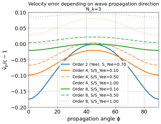
Regarding the numerical anisotropy of the phase velocity, using higher order finite differences for the approximation of spatial derivatives significantly improves the dispersion properties of the solver. Most notably, the velocity anisotropy reduces and the dependence of phase velocity on sampling reduces, too. Yet higher order solvers still feature dispersion. As shown in the following picture, its effect is, however, not reduction of phase velocity but increase of phase velocity beyond the physical vacuum speed of light. But this can be tweaked by reducing the time step relative to the limit set by the stability criterion.

Note, it is generally not a good idea to reduce the time step in Yee’s method significantly below the stability criterion as this increases the absolute phase velocity error. See the following figure,
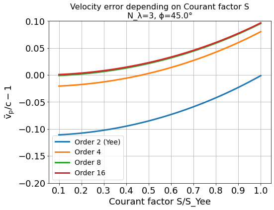
from which the optimum Courant factor \(S=c\Delta t / \Delta\) can be read off for a 2D, square mesh, too.
An important conclusion from the above figures showing velocity error over sampling is, that a higher order solver, with a larger mesh spacing and a smaller time step than given by the above stability limit, produces physically more accurate results than the standard Yee solver operating with smaller mesh spacing and a time step close to the stability limit.
That is, it can be beneficial not only in terms of physical accuracy, but also in terms of memory complexity and time to solution, to chose a higher order solver with lower spatial resolution and increased time sampling relative to the stability limit. Memory complexity scales with number of cells \(N_\mathrm{cells}\) required to sample a given volume \(N_\mathrm{cells}^d\), where \(d=2,3\) is the dimension of the simulation domain, which decreases for larger cells. Time to solution scales with the time step and this can be larger with solvers of higher order compared to the Yee solver with comparable dispersion properties (which requires a smaller cell size than the arbitrary order solver) since the time step is limited by the stability condition which scales with cell size. Since the cell size can be larger for arbitrary order solvers, the respective time step limit given by the stability condition is larger and operating with a time step ten times smaller than the limit might still result in a larger step than those of the comparable Yee solver. Finally, physical accuracy is increased by the reduction of the impact of dispersion effects.
Usage
The field solver can be chosen and configured in fieldSolver.param.
Substepping
Any field solver can be combined with substepping in time. In this case, each iteration of the main PIC loop involves multiple invocations of the chosen field solver. Substepping is fully compatible with other numerics, such as absorbers, incident field, laser generation. A substepping field solver has the same orders of accuracy in spatial and time steps as the base solver.
A user sets main PIC time step value as usual in simulation.param, and selects the number of field solver substeps via template argument T_numSubsteps. Field solver will internally operate with \(\Delta t_{sub} = \Delta t / \mathrm{T\_numSubsteps}\). Solver properties including the Courant-Friedrichs-Lewy condition are then expressed with \(\Delta t_{sub}\), which is less restricting. However, regardless of field solver and substepping PIConGPU also limits its main time step to
for 3D; for 2D the requirement is similar but does not involve \(\Delta z\).
Still, with substepping solver a user could sometimes increase the value of \(\Delta t\) used. Consider a simplified case of \(\Delta x = \Delta y = \Delta z\), and Yee solver with a time step value near the Courant-Friedrichs-Lewy condition threshold \(\Delta t_{base} = 0.995 \frac{\Delta x}{c \sqrt 3}\). Raising the main time step to \(t_{max}\) and substepping by 2 would make the field solver have \(\Delta t_{sub} < \Delta t_{base}\) thus satisfying the Courant-Friedrichs-Lewy condition and providing slightly better resolution. Whether this approach is applicable then depends on whether \(t_{max}\) sufficiently resolves plasma wavelength and other time scales in the rest of the PIC loop.
References
T.Zh. Esirkepov, Exact charge conservation scheme for particle-in-cell simulation with an arbitrary form-factor, Computer Physics Communications 135.2 (2001): 144-153, https://doi.org/10.1016/S0010-4655(00)00228-9
M. Ghrist, High-Order Finite Difference Methods for Wave Equations, PhD thesis (2000), Department of Applied Mathematics, University of Colorado
R. Lehe et al. Numerical growth of emittance in simulations of laser-wakefield acceleration, Physical Review Special Topics-Accelerators and Beams 16.2 (2013): 021301.
A. Taflove, S.C. Hagness Computational electrodynamics: the finite-difference time-domain method Artech house (2005)
K.S. Yee, Numerical solution of initial boundary value problems involving Maxwell’s equations in isotropic media, IEEE Trans. Antennas Propagat. 14, 302-307 (1966)