Species translation

In PIConGPU (and PIC-codes in general) “Species” is a catch-all term for all things particles; it is defined rather losely and used differently in different contexts.

Generally, a “species” is a set of macroparticles in a simulation which are initialized from a common parameter set.

A macroparticle is a representation of a varying number of simulated (“real”) particles.

For PyPIConGPU a species consists of a set constant properties (same for each macroparticle, “flags”) and a set of variable properties (attributes, exists for every macroparticle, but may have a different value). Each attribute is initialized by exactly one operation.

This results in this UML class diagram.

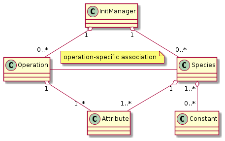
Fig. 36 Final relationships of species-related classes

In particular, the name is part of this common parameter set, as well as the profile where these particles are placed. If you want to initialize the same type of particles (e.g. the same substance) with a different profile, a second species has to be created.

This document describes how species are translated from PICMI, via an intermediate PyPIConGPU-only representation, to executable PIConGPU .param files. For the general process of translation please refer to the respective documentation section. The process is outlined back-to-front here, i.e. starting with the desired PIConGPU result, deriving the PyPIConGPU representation from that and explaining some PICMI details in the end.

Neither PICMI nor PIConGPU species declaration are introduced in detail, please familiarize yourself with both.

Code Generation

A species is directly associated to two code sections:

1. A species definition, declaring a C++ species type, placed inside speciesDefinition.param.

2. A species initialization, creating and initializing the attributes of the species’ macroparticles, placed inside the init pipeline of speciesInitialization.param.

Particles of a species have different properties, which fall into one of two categories:

• Constants (Flags in PIConGPU lingo): Properties that apply to all (macro-) particles and can’t be changed for each macroparticle

  • typically matter constants, e.g. number of protons, mass, charge

  • but also: used pusher, particle shape, etc.

  • initialized in speciesDefinition.param

• Attributes: Properties that can be different from macroparticle to macroparticle

  • most importantly the position

  • other changing/changeable properties, e.g. momentum, number of bound electrons

  • existence declared in speciesDefinition.param

  • initialized in speciesInitialization.param (actual initialization typically loaded from other files, e.g. density.param)

The constants are stored purely in the type definition. Attributes must be enabled for their respective species in their type definition, but they are set in the init pipeline.

A list of flags and a list of attributes is passed directly from PyPIConGPU, which makes code generation rather straightforward.

The initpipeline is expressed by a set of operations, which by definition have no interdependencies. For more details on operations please refer to the next section.

Note that while the init operations have no inherent order, they are generated in such a way that macroparticles are placed before any other attributes are set.

When reading the generated code note that while all operations are referred to in the initpipeline, they are typically defined in a separate file. (This is more in line with the native PIConGPU configuration.)

Architecture of PyPIConGPU Representation

The PyPIConGPU representation of species initialization uses the concepts species, constant, attribute, operation and init manager and defines their relationships.

• The init manager is the global context managing the entire lifecycle.

  • …performs all checks between objects that are not directly associated to one another

• A species is a type of macroparticles sharing the same properties.

  • …has a (mandatory) name

  • …has a list of constants and a list of attributes

  • …will only be considered “valid” if position and momentum attributes are set

  • …has at most one of each constant (type)

  • …has at most one of each attribute (type)

• A constant is a unmodifiable property shared among all macroparticles of a species (flag in PIConGPU lingo)

  • …are for example charge and mass.

  • …carries its value inside its object representation

  • …is owned by a species

  • …may depend on other species being present (during code generation)

• An attribute is a property which every macroparticle has, but each may have a different value

  • …are for example position and weighting

  • …object only contains a name

  • …is exclusive to a species

  • …is provided (generated) by an operation, which also sets it (inside of PIConGPU); in other words:

  • …is “in exclusive custody” of exactly one operation.

• An operation initializes a set of attributes for a set of species

  • …is independent from all other operations

  • …gets passed its parameters and affected species in a custom way (i.e. there is no globally unified way to pass parameters to operations)

  • …provides and sets a attributes for its species

  • …may depend on constants.

  • …must NOT depend on other attributes/operations.

This leads to some notable conclusions:

An attribute is always managed exclusively by exactly one operation. The purpose of this is it to make it easy to detect conflicts between operations, and at the same time making it very clear what caused the value of an attribute.

Therefore, if two attributes depend on each other, they must be set in the same operation. E.g., when placing ions and their electrons, both are created from the same SimpleDensity operation.

Also, if multiple factors determine an attribute, they must be specified inside of the same operation: E.g. the momentum is influenced by both temperature and drift, hence they are properties of the SimpleMomentum operation.

We somewhat jokingly refer to this setup as the “grand unified theory of species”.

Lifecycle

The core idea behind this architecture is to associate every attribute (of one species) with exactly one operation.

This has two main advantages:

(1) operations are independent of one another, and

(2) the initialization can be traced back to exactly one operation.

To ensure this, the species initialization follows this lifecycle:

1. initialize species, constants, and operations

2. check if this setup is valid

3. operations create attributes and prebook them for some species

4. these prebooked attributes are checked, if no conflicts are found they are added to their species

For the implementation of this process, please see picongpu.pypicongpu.species.InitManager.bake().

The generating script creates this setup:

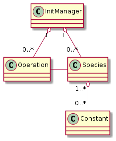
Fig. 37 Setup as created by PyPIConGPU (before Operations have been applied)

After all checks have passed, the operations may pre-book the attributes they want to create. Pre-Booking is performed in picongpu.pypicongpu.species.operation.Operation.prebook_species_attributes() by creating the intended Attribute objects (one per species) and storing the intended association into the Operation.attributes_by_species.

Pre-Booking results in this intermediate connection:

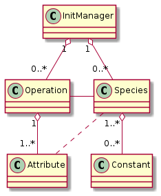
Fig. 38 classes with prebooked association

After these pre-booked species-attribute connections have been checked, they are baked, i.e. applied into the final model:

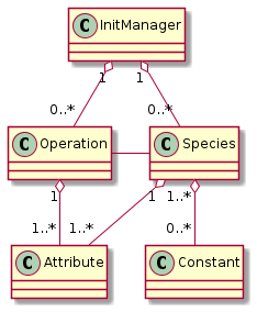
Fig. 39 final (baked) species-related classes

From these classes the code generation can simply derive:

• a list of species, and for each species

  • its constants

  • required attributes

• a list of operations

Note that the some associations from the model above are lost when translating to JSON for code generation, e.g. which operation initializes which attribute.

Checks

Constants, Attributes, and Operations may have various dependencies. All possible dependencies are listed here:

• Species may depend on:

  • Nothing: Species are passive, and are manipulated by multiple Operations.

  • As a sanity check species require Position and Momentum attributes (as hard-coded checks). This is not because the model requires it, but because species without these make no sense in PIC implementations.

• Attributes may depend on:

  • Nothing: Attributes are passive, and are manipulated by exactly one Operation.

• Constants may depend on:

  • (not-finalized) Species objects: E.g. ions may depend on their electrons. These dependencies modify the order in which the species are rendered to code.

  • (existence of) Attribute types: E.g. ionizers depend on the attribute BoundElectrons. The Operation which sets the Attribute is not visible to the check.

  • (existence of) Constant types: E.g. ionizers depend on the constant ElementProperties (which contains the ionization levels). The value of these constants is not visible to the check.

• Operations may depend on:

  • their Species: Note that at this point the Species do not have any Attributes added. (Accessing the Attributes will result in an error.)

  • (through their Species) these Species’ Constants: These are the Attribute objects, i.e. their value can be read (and checked against).

Other dependencies are forbidden by design. Notably, this includes Operation-Operation and Operation-Attribute dependencies, because Operations are independent from one another.

Note

Errorneous (circular) dependencies are checked by the init manager.

All checks are invoked when applying the Operations in the init manager’s bake() method (see also: Lifecycle). (For their implementation details please refer to the respective base classes.)

Constants

PyPIConGPU Constant objects follow the concept of a constant property, instead of mirroring the PIConGPU Species Flags 1-to-1.

E.g., the Constant ElementProperties is translated to atomic numbers and ionization energies.

(Note: Mass and Charge are treated as separate constants, even if they are element properties too.)

Constants may depend on other species, which is required due to the C++ syntax: Forward declarations (referring to to-be-defined things, in this case species) are not possible for this case (template programming), so the order of the code generation matters. This order is governed by the Constant-Species dependencies and handled by the init manager.

Attributes

Attributes are enabled by adding them to the type definition in PIConGPU. Their values are set in the init pipeline.

The PyPIConGPU species model (see: Architecture of PyPIConGPU Representation) ties Attributes strongly to Operations: An Attribute is always initialized (handled, created) by exactly one Operation. Hence, Attributes are never created directly, but only ever through Operations (see: Lifecycle).

Operations

Operations create and initialize Attributes exclusively, i.e. one Attribute of a Species can only ever be initialized by exactly one Operation.

There is no unified way in which Operations must accept their arguments, i.e. an Operation must define its own interface how Species and arguments must be passed.

Operations are the intended way how dependencies between Attribute values should be expressed: If two Attributes are related, they must be initialized by the same Operation. For that, the Operation may depend on Constants of these Species (in check_preconditions()), but it must NOT modify these Constants.

During the code generation these Operations may result in any number of “Functors” in the init pipeline.

The init manager translates the Operations to JSON, creating a dictionary

{
    "op_type1": [ "OP1", "OP2" ],
    "op_type2": [ "OP3" ],
    "op_type3": []
}

For this every type of Operation must be registered with a name in _get_serialized() in the init manager (and the respective schema).

Conceptually Operations are independent from other Operations. However, for code generation an inherent order is required, which implicitly introduces an order between these Operations. Yet, this order is only required for placing macroparticles (particles must be created before they can be modified) – for all other cases it is ignored.

The concept of Operations aims to move the species initialization closer to a declarative description (“momentum is x”), instead of PIConGPU’s procedural description (”set momentum to x”).

Note

The purpose of this is to enable traceability and thereby error handling. A procedural description is very powerful, but quickly runs into the Halting Problem, rendering any programmatic handling (besides execution) impossible. (This includes any manipulation, checking or predicting results.)

In many cases PIConGPU’s functors from the init pipeline can be translated to a single operation, however this is not the case for all examples:

• setting the number of bound electrons for ions

  • Attributes: boundElectrons

  • PIConGPU: set bound electrons functor (implementation of Free functor)

  • PyPIConGPU: BoundElectrons Operation

• not placing a species itself (e.g. electron species)

  • Attributes: position<position_pic>, weighting

  • PIConGPU: leave init pipeline empty, but add position<position_pic> Attribute

  • PyPIConGPU: NotPlaced Operation

• setting the momentum, composed of drift and temperature

  • Attributes: momentum

  • PIConGPU: set drift, then add temperature in second operation

  • PyPIConGPU: SimpleMomentum Operation (which accepts both drift and temperature)

• placing multiple species together (see also next section)

  • Attributes: position<position_pic>, weighting

  • PIConGPU: CreateDensity for first species, then Derive all other species

  • PyPIConGPU: SimpleDensity Operation, which accepts a list of Species

Placement

The Placement describes the creation of macroparticles. (Which differs from all other Operations, because they only modify existing macroparticles.)

Ultimately, the particle placement expresses where macroparticles with which weighting (number of represented real particles) should be placed.

For this, the following components may be specified:

PICMI term (PIConGPU term)

• particle distribution (density profile): specifies density by location

  • function w.r.t. x, y, z of global coordinate system

  • typically expressed relative to base density

• density scale (density ratio): modifies density

  • scalar factor, multiplied with particle distribution

• particle layout (particle position): specifies position and number of macro particles inside the cell

  • typically random or fixed to grid positions

Note that there are two steps in deriving the placement of particles from the density. The density, i.e. number of (real) particles per volume is given by a particle distribution (density profile). This profile is multiplied with the density scale (density ratio) and then

1. discretized, i.e. for every cell the average density/the number of particles is computed

2. Based on the particle layout (particle position) a certain number of macroparticles are placed at a certain position inside every cell.

3. The weighting of these macroparticles is adjusted to match the computed density. If the weighting is below a configurable threshold, particles will be deleted.

This document uses the following terms:

used here	PIConGPU	PICMI	description
profile	density profile	particle distribution	description of number of particles per unit of volume
ratio	density ratio	density scale	scalar factor applied to profile (modifies the number of particles represented by one macroparticle)
layout	particle position	particle layout	positioning of macroparticles within a cell

The term “placement” refers to the entire process of placing macroparticles from parameters to final positioning.

Initializing Multiple Species

Some species are to be created together, e.g. ions and their respective electrons. Though, in general, species are treated separately during initialization.

The main purpose of this grouping is to join particles in such a way, that in total their charge is (locally) neutral. See: Quasi-Neutral Initialization

For the purposes of this document, species might be related as follows:

• If two (or more) species are related in such a way that their purpose is to bring the total (local) charge to a neutral level, they are to be derived from each other.

• If the species are not related in such a way, they are to be treated separately.

PICMI initializes all species equally, i.e. simply stores a list of all species to be initialized: The distinction above is not made explictly: For PICMI, species that are to be derived from each other simply end up at the same place (and can thus neutralize each other) after applying all initialization of values & position (profile, layout, ratio).

PIConGPU on the other hand uses a different approach. There, particles that are to be derived from each other are initialized in order: Only the first species (of the group to be derived) is placed by a placing algorithm, all other derived species have their position simply copy-pasted from this first. (If necessary the scalar density scale is adjusted.)

PIConGPU here is more efficient than (naive) PICMI, because instead of placing all particles s.t. the positions are equal for two (or more) species (in which case they are derived), only the initial positions are calculated – and all derived species’ positions are made to be equal.

This schema of separate initialization, yet same final positioning can not be recreated in PIConGPU. The problem lies in the random layout: When calling the same random layout in PIConGPU twice, the results do not match. Therefore, particles that are to be grouped together are derived from each other in PIConGPU-native setups.

There are very good reasons of the implementation to do that: (1) It is more efficient to copy positions instead of generating them twice. (2) Due to the parallel nature of PIConGPU, a random placement is not reproducable. (Not reasonably in practical scenarios at least: In particular, it is very difficult to keep the RNG state in sync==reproducable across many processes, across many different algorithms, and across all supported architectures.)

The implicit grouping in PICMI has to be made explicit before translating the particle initialization to PIConGPU. For that we consider the following cases to decide if two species are to be derived or treated separately, depending if their initialization parameters (profile, layout, ratio) are different or equal.

profile	layout	ratio	behavior
different	different	different	treat separately
different	different	equal	treat separately
different	equal	different	treat separately
different	equal	equal	treat separately
equal	different	different	treat separately
equal	different	equal	treat separately
equal	equal	different	derive
equal	equal	equal	derive

This grouping is performed during the translation from PICMI to PyPIConGPU. Profiles/Layouts are considered equal if they are == equal. For PICMI, == equality is the same to is (object identity), i.e. two species have the same profile (particle distribution) if they use the same particle distribution object. (PICMI may redefine == in the future.)

In PyPIConGPU Species that are to be derived are grouped into the same SimpleDensity Operation.

Ratios are stored in Constants (PIConGPU species flags), and the species with the lowest ratio is placed first to make sure the minimum weighting is always respected. Note that the first species is not required to use a ratio of one, which is handled properly by PIConGPU (both during placement and copying).

Notes

Seeds

Seeds are not supported and entirely ignored by PyPIConGPU.

Use Ratios over Profiles!

The density is defined by a profile multiplied by a ratio. Hence, in theory the following two are equal:

• Ratio 1, Profile f(x,y,z) = 6e24 + x * 2e23

• Ratio 2, Profile f(x,y,z) = 3e24 + x * 1e23

However, this is to be discouraged:

Using a new profile (1) has to be computed for every cell and (2) disables the option to detect species placed together.

Reusing an existing profile (1) is more efficient (reuses previous results) and (2) allows to detect species placed together.

Ratio Handling

Ratios are scalar factors applied to profiles.

Profiles are expressed that they are valid with a ratio of one. By specifying a different PIConGPU density ratio (in the species flags) the PIConGPU CreateDensity functor in the init pipeline will adjust the weighting accordingly.

The subsequent Derive functors to copy the species location respect the ratios of the respective species (specifically: the ratio of their ratios), so no additional measures are required.

Electron Resolution

PIConGPU requires an explicit species to be used for electrons, whereas this is not possible to specify with PICMI.

The user can either explicitly set the electron species by providing picongpu_ionization_electrons to the PICMI species, or the PICMI translation will try to guess the used electron species. If there is exactly one electron species it will be used, if there is no electron species one will be added, and if there are two or more electron species an error will be raised.

Example

This example shows the initialization of a constant density of Helium with one bound electron. For the sake of the example the ratio is 0.5. The PICMI initialization is:

PICMI

uniform_dist = picmi.UniformDistribution(density=8e24,
                                         rms_velocity=[1e5, 1e5, 1e5])
species_helium = picmi.Species(name="helium",
                               particle_type="He",
                               charge_state=1,
                               density_scale=0.4,
                               initial_distribution=uniform_dist)

# init of sim omitted

random_layout = picmi.PseudoRandomLayout(n_macroparticles_per_cell=2)
sim.add_species(species_helium, random_layout)

For which an additional electron species is added, equivalent to:

electrons = picmi.Species(name="e",
                          particle_type="electron")
sim.add_species(electrons, None)

PyPIConGPU

This translated to these PyPIConGPU objects (simplified, some helper objects are omitted):

Warning

This is a UML object diagram, not a (generally more common) class diagram as above. (Boxes here are objects instead of classes.)

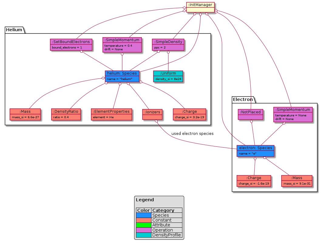
Fig. 40 example setup as translated by PICMI before Baking

After attribute creation, prebooking, checking and finally baking, this results in these objects:

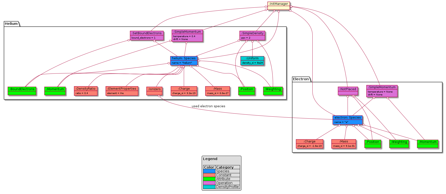
Fig. 41 example setup after baking attributes

Rendering JSON Representation

From this, the following (abbreviated) JSON representation is derived:

ALL CAPS strings are placeholders for full (complex) objects

{
    "species": [
        {
            "name": "e",
            "typename": "species_e",
            "attributes": [
                {"picongpu_name": "position<position_pic>"},
                {"picongpu_name": "weighting"},
                {"picongpu_name": "momentum"}
            ],
            "constants": {
                "mass": {"mass_si": 9.1093837015e-31},
                "charge": {"charge_si": -1.602176634e-19},
                "density_ratio": null,
                "ionizers": null,
                "element_properties": null
            }
        },
        {
            "name": "helium",
            "typename": "species_helium",
            "attributes": [
                {"picongpu_name": "position<position_pic>"},
                {"picongpu_name": "weighting"},
                {"picongpu_name": "momentum"},
                {"picongpu_name": "boundElectrons"}
            ],
            "constants": {
                "mass": {"mass_si": 6.64647366797316e-27},
                "charge": {"charge_si": 3.204353268e-19},
                "density_ratio": {"ratio": 0.4},
                "ionizers": {"electron_species": "ELECTRON SPECIES OBJECT"},
                "element_properties": {
                    "element": {
                        "symbol": "He",
                        "picongpu_name": "Helium"
                    }
                }
            }
        }
    ],
    "operations": {
        "simple_density": ["SIMPLE DENSITY OBJECT"],
        "simple_momentum": [
            {
                "species": "HELIUM SPECIES OBJECT",
                "temperature": {"temperature_kev": 0.41484025711818995},
                "drift": null
            },
            {
                "species": "ELECTRON SPECIES OBJECT",
                "temperature": null,
                "drift": null
            }
        ],
        "set_bound_electrons": [
            {
                "species": "HELIUM SPECIES OBJECT",
                "bound_electrons": 1
            }
        ]
    }
}

Generated Code

Ultimately rendering this code (reformatted for reading):

speciesDefinition.param:

value_identifier(float_X, MassRatio_species_e,
                9.1093837015000008e-31 / SI::BASE_MASS_SI);
value_identifier(float_X, ChargeRatio_species_e,
                -1.6021766339999999e-19 / SI::BASE_CHARGE_SI);

using ParticleFlags_species_e = MakeSeq_t<
    massRatio<MassRatio_species_e>, chargeRatio<ChargeRatio_species_e>,

    particlePusher<UsedParticlePusher>, shape<UsedParticleShape>,
    interpolation<UsedField2Particle>, current<UsedParticleCurrentSolver>>;

using ParticleAttributes_species_e =
    MakeSeq_t<position<position_pic>, weighting, momentum>;

using species_e = Particles<PMACC_CSTRING("e"), ParticleFlags_species_e,
                            ParticleAttributes_species_e>;


value_identifier(float_X, MassRatio_species_helium,
                6.6464736679731602e-27 / SI::BASE_MASS_SI);
value_identifier(float_X, ChargeRatio_species_helium,
                3.2043532679999998e-19 / SI::BASE_CHARGE_SI);
value_identifier(float_X, DensityRatio_species_helium, 0.40000000000000002);

using ParticleFlags_species_helium = MakeSeq_t<
    massRatio<MassRatio_species_helium>,
    chargeRatio<ChargeRatio_species_helium>,
    densityRatio<DensityRatio_species_helium>,

    ionizers<MakeSeq_t<particles::ionization::BSI<
                        species_e, particles::ionization::current::None>,
                    particles::ionization::ADKCircPol<
                        species_e, particles::ionization::current::None>,
                    particles::ionization::ThomasFermi<species_e>>>,

    atomicNumbers<ionization::atomicNumbers::Helium_t>,
    ionizationEnergies<ionization::energies::AU::Helium_t>,

    particlePusher<UsedParticlePusher>, shape<UsedParticleShape>,
    interpolation<UsedField2Particle>, current<UsedParticleCurrentSolver>>;

using ParticleAttributes_species_helium =
    MakeSeq_t<position<position_pic>, weighting, momentum, boundElectrons>;

using species_helium =
    Particles<PMACC_CSTRING("helium"), ParticleFlags_species_helium,
            ParticleAttributes_species_helium>;

using VectorAllSpecies = MakeSeq_t<species_e, species_helium>;

The operations result in this speciesInitialization.param:

using InitPipeline = boost::mp11::mp_list<
    /**********************************/
    /* phase 1: create macroparticles */
    /**********************************/

    CreateDensity<densityProfiles::pypicongpu::init_species_helium,
                  startPosition::pypicongpu::init_species_helium,
                  species_helium>,

    /*********************************************/
    /* phase 2: adjust other attributes (if any) */
    /*********************************************/

    // *adds* temperature, does *NOT* overwrite
    Manipulate<manipulators::pypicongpu::AddTemperature_species_helium,
               species_helium>,

    Manipulate<manipulators::pypicongpu::PreIonize_species_helium,
               species_helium>,

    // does nothing -- exists to catch trailing comma left by code generation
    pypicongpu::nop>;

Utilizing this density definition from density.param:

/**
* generate the initial macroparticle position for species "helium"
* (species_helium)
*/
struct init_species_helium_functor {
    HDINLINE float_X operator()(const floatD_64 &position_SI,
                                const float3_64 &cellSize_SI) {
        return 7.9999999999999999e+24 / SI::BASE_DENSITY_SI;
    }
};

using init_species_helium =
    FreeFormulaImpl<init_species_helium_functor>;