Particle-in-Cell Simulations for the Exascale Era
PIConGPU is a fully relativistic, manycore, 3D3V and 2D3V particle-in-cell (PIC) code. The PIC algorithm is a central tool in plasma physics. It describes the dynamics of a plasma by computing the motion of electrons and ions in the plasma based on the Vlasov-Maxwell system of equations.
How to Read This Document
Generally, to get started follow the manual pages in order. Individual chapters are based on the information in the chapters before. In case you are already fluent in compiling C++ projects and HPC, running PIC simulations or scientific data analysis, feel free to jump the respective sections.
The online version of this document is versioned and shows by default the manual of the last stable version of PIConGPU. If you are looking for the latest development version, click here.
Note
We are migrating our wiki to this manual, but some pages might still be missing. We also have an official homepage .
Note
Are you looking for our latest Doxygen docs for the API?
Installation
Introduction
Section author: Axel Huebl
Installing PIConGPU means installing C++ libraries that PIConGPU depends on and setting environment variables to find those dependencies. The first part is usually the job of a system administrator while the second part needs to be configured on the user side.
Depending on your experience, role, computing environment and expectations for optimal hardware utilization, you have several ways to install and select PIConGPU’s dependencies. Choose your favorite install and environment management method below, young padawan, and follow the corresponding sections of the next chapters.
Ways to Install
Choose one of the installation methods below to get started.
Load Modules
On HPC systems and clusters, software is usually provided by system administrators via a module system (e.g. [modules], [Lmod]).
In case our software dependencies are available, we usually create a file in our $HOME named <queueName>_picongpu.profile.
It loads according modules and sets helper environment variables.
Important
For many HPC systems we have already prepared and maintain an environment which will run out of the box. See if your system is in the list so you can skip the installation completely!
Spack
[Spack] is a flexible package manager that can build and organize software dependencies. It can be configured once for your hardware architecture to create optimally tuned binaries and provides modulefile support (e.g. [modules], [Lmod]). Those auto-build modules manage your environment variables and allow easy switching between versions, configurations and compilers.
Build from Source
You choose a supported C++ compiler and configure, compile and install all missing dependencies from source. You are responsible to manage the right versions and configurations. Performance will be ideal if architecture is chosen correctly (and/or if built directly on your hardware). You then set environment variables to find those installs.
Conda
We currently do not have an official conda install (yet). Due to pre-build binaries, performance could be not ideal and HPC cluster support (e.g. MPI) might be very limited. Useful for small desktop or single-node runs.
Nvidia-Docker
Not yet officially supported [nvidia-docker], but we already provide a Dockerfile to get started.
Performance might be not ideal if the image is not built for the specific local hardware again.
Useful for small desktop or single-node runs.
We are also working on Singularity images.
References
- Spack
T. Gamblin and contributors. A flexible package manager that supports multiple versions, configurations, platforms, and compilers, SC ‘15 Proceedings of the International Conference for High Performance Computing, Networking, Storage and Analysis (2015), DOI:10.1145/2807591.2807623, https://github.com/spack/spack
- modules(1,2)
J.L. Furlani, P.W. Osel. Abstract Yourself With Modules, Proceedings of the 10th USENIX conference on System administration (1996), http://modules.sourceforge.net
- Lmod(1,2)
R. McLay and contributors. Lmod: An Environment Module System based on Lua, Reads TCL Modules, Supports a Software Hierarchy, https://github.com/TACC/Lmod
- nvidia-docker
Nvidia Corporation and contributors. Build and run Docker containers leveraging NVIDIA GPUs, https://github.com/NVIDIA/nvidia-docker
Instructions
Section author: Axel Huebl
As explained in the previous section, select and follow exactly one of the following install options.
See also
You will need to understand how to use the terminal.
Warning
Our spack package is still in beta state and is continuously improved. Please feel free to report any issues that you might encounter.
Spack
Section author: Axel Huebl
Preparation
First install spack itself via:
# get spack
git clone https://github.com/spack/spack.git $HOME/src/spack
# activate the spack environment
source $HOME/src/spack/share/spack/setup-env.sh
# install a supported compiler
spack compiler list | grep -q gcc@7.3.0 || spack install gcc@7.3.0 && spack load gcc@7.3.0 && spack compiler add
# add the PIConGPU repository
git clone https://github.com/ComputationalRadiationPhysics/spack-repo.git $HOME/src/spack-repo
# add the new repo to spack
spack repo add $HOME/src/spack-repo
Note
When you open a terminal next time or log back into the machine, make sure to activate the spack environment again via:
source $HOME/src/spack/share/spack/setup-env.sh
Install
The installation of the latest version of PIConGPU is now as easy as:
spack install picongpu %gcc@7.3.0
Use PIConGPU
PIConGPU can now be loaded with
spack load picongpu
For more information on variants of the picongpu package in spack run spack info picongpu and refer to the official spack documentation.
Note
PIConGPU can also run without a GPU!
For example, to use our OpenMP backend, just add backend=omp2b to the two commands above:
spack install picongpu backend=omp2b
spack load picongpu backend=omp2b
Note
If the install fails or you want to compile for CUDA 9.2, try using GCC 5.5.0:
spack compiler list | grep gcc@5.5.0 | spack install gcc@5.5.0 && spack load gcc@5.5.0 && spack compiler add
spack install picongpu %gcc@5.5.0
spack load picongpu %gcc@5.5.0
See also
You will need to understand how to use the terminal.
Warning
Docker images are experimental and not yet fully automated or integrated.
Docker
Section author: Axel Huebl
Preparation
First install nvidia-docker for your distribution. Use version 2 or newer.
Install
The download of a pre-configured image with the latest version of PIConGPU is now as easy as:
docker pull ax3l/picongpu
Use PIConGPU
Start a pre-configured LWFA live-simulation with
docker run --runtime=nvidia -p 2459:2459 -t ax3l/picongpu /bin/bash -lc start_lwfa
# open firefox and isaac client
or just open the container and run your own:
docker run --runtime=nvidia -it ax3l/picongpu
Note
PIConGPU can also run without a GPU! We will provide more image variants in the future.
See also
You will need to understand how to use the terminal.
Note
This section is a short introduction in case you are missing a few software packages, want to try out a cutting edge development version of a software or have no system administrator or software package manager to build and install software for you.
From Source
Section author: Axel Huebl
Don’t be afraid, young physicist, self-compiling C/C++ projects is easy, fun and profitable!
Building a project from source essentially requires three steps:
configure the project and find its dependencies
compile the project
install the project
All of the above steps can be performed without administrative rights (“root” or “superuser”) as long as the install is not targeted at a system directory (such as /usr) but inside a user-writable directory (such as $HOME or a project directory).
Preparation
In order to compile projects from source, we assume you have individual directories created to store source code, build temporary files and install the projects to:
# source code
mkdir $HOME/src
# temporary build directory
mkdir $HOME/build
# install target for dependencies
mkdir $HOME/lib
Note that on some supercomputing systems, you might need to install the final software outside of your home to make dependencies available during run-time (when the simulation runs). Use a different path for the last directory then.
What is Compiling?
Note
This section is not yet the installation of PIConGPU from source. It just introduces in general how one compiles projects.
If you like to skip this introduction, jump straight to the dependency install section.
Compling can differ in two principle ways: building inside the source directory (“in-source”) and in a temporary directory (“out-of-source”). Modern projects prefer the latter and use a build system such as [CMake].
An example could look like this
# go to an empty, temporary build directory
cd $HOME/build
rm -rf ../build/*
# configurate, build and install into $HOME/lib/project
cmake -DCMAKE_INSTALL_PREFIX=$HOME/lib/project $HOME/src/project_to_compile
make
make install
Often, you want to pass further options to CMake with -DOPTION=VALUE or modify them interactively with ccmake . after running the initial cmake command.
The second step which compiles the project can in many cases be parallelized by make -j.
In the final install step, you might need to prefix it with sudo in case CMAKE_INSTALL_PREFIX is pointing to a system directory.
Some older projects often build in-source and use a build system called autotools. The syntax is still very similar:
# go to the source directory of the project
cd $HOME/src/project_to_compile
# configurate, build and install into $HOME/lib/project
configure --prefix=$HOME/lib/project
make
make install
One can usually pass further options with --with-something=VALUE or --enable-thing to configure.
See configure --help when installing an autotools project.
That is all on the theory of building projects from source!
Now Start
You now know all the basics to install from source. Continue with the following section to build our dependencies.
References
- CMake
Kitware Inc. CMake: Cross-platform build management tool, https://cmake.org/
If anything goes wrong, an overview of the full list of PIConGPU dependencies is provided in section Dependencies.
After installing, the last step is the setup of a profile.
See also
You will need to understand how to use the terminal, what are environment variables and please read our compiling introduction.
Note
If you are a scientific user at a supercomputing facility we might have already prepared a software setup for you. See the following chapter if you can skip this step fully or in part by loading existing modules on those systems.
Dependencies
Section author: Axel Huebl
Overview

Overview of inter-library dependencies for parallel execution of PIConGPU on a typical HPC system. Due to common binary incompatibilities between compilers, MPI and boost versions, we recommend to organize software with a version-aware package manager such as spack and to deploy a hierarchical module system such as lmod. An Lmod example setup can be found here.
Requirements
Mandatory
gcc
5.5 - 10.0 (if you want to build for Nvidia GPUs, supported compilers depend on your current CUDA version)
CUDA 9.2 - 10.0: Use gcc 5.5 - 7
CUDA 10.1/10.2: Use gcc 5.5 - 8
CUDA 11.x: Used gcc 5.5 - 10.0
note: be sure to build all libraries/dependencies with the same gcc version; GCC 5 or newer is recommended
Debian/Ubuntu:
sudo apt-get install gcc-5 g++-5 build-essentialsudo update-alternatives --install /usr/bin/gcc gcc /usr/bin/gcc-5 60 --slave /usr/bin/g++ g++ /usr/bin/g++-5
Arch Linux:
sudo pacman --sync base-develif the installed version of gcc is too new, compile an older gcc
Spack:
spack install gcc@5.5.0make it the default in your packages.yaml or suffix all following
spack installcommands with a space and%gcc@5.5.0
CMake
3.15.0 or higher
Debian/Ubuntu:
sudo apt-get install cmake file cmake-curses-guiArch Linux:
sudo pacman --sync cmakeSpack:
spack install cmake
MPI 2.3+
OpenMPI 1.7+ / MVAPICH2 1.8+ or similar
for running on Nvidia GPUs, perform a GPU aware MPI install after installing CUDA
Debian/Ubuntu:
sudo apt-get install libopenmpi-devArch Linux:
sudo pacman --sync openmpiSpack:
GPU support:
spack install openmpi+cudaCPU only:
spack install openmpi
environment:
export MPI_ROOT=<MPI_INSTALL>as long as CUDA awareness (
openmpi+cuda) is missing:export OMPI_MCA_mpi_leave_pinned=0
zlib
Debian/Ubuntu:
sudo apt-get install zlib1g-devArch Linux:
sudo pacman --sync zlibSpack:
spack install zlibfrom source:
./configure --prefix=$HOME/lib/zlibmake && make install
environent: (assumes install from source in
$HOME/lib/zlib)export ZLIB_ROOT=$HOME/lib/zlibexport LD_LIBRARY_PATH=$ZLIB_ROOT/lib:$LD_LIBRARY_PATHexport CMAKE_PREFIX_PATH=$ZLIB_ROOT:$CMAKE_PREFIX_PATH
boost
1.65.1 - 1.74.0 (
program_options,filesystem,system,math,serializationand header-only libs, optional:fiberwithcontext,thread,chrono,atomic,date_time)Debian/Ubuntu:
sudo apt-get install libboost-program-options-dev libboost-filesystem-dev libboost-system-dev libboost-thread-dev libboost-chrono-dev libboost-atomic-dev libboost-date-time-dev libboost-math-dev libboost-serialization-dev libboost-fiber-dev libboost-context-devArch Linux:
sudo pacman --sync boostSpack:
spack install boostfrom source:
curl -Lo boost_1_65_1.tar.gz https://dl.bintray.com/boostorg/release/1.65.1/source/boost_1_65_1.tar.gztar -xzf boost_1_65_1.tar.gzcd boost_1_65_1./bootstrap.sh --with-libraries=atomic,chrono,context,date_time,fiber,filesystem,math,program_options,serialization,system,thread --prefix=$HOME/lib/boost./b2 cxxflags="-std=c++11" -j4 && ./b2 install
environment: (assumes install from source in
$HOME/lib/boost)export BOOST_ROOT=$HOME/lib/boostexport LD_LIBRARY_PATH=$BOOST_ROOT/lib:$LD_LIBRARY_PATH
git
1.7.9.5 or higher
Debian/Ubuntu:
sudo apt-get install gitArch Linux:
sudo pacman --sync gitSpack:
spack install git
rsync
Debian/Ubuntu:
sudo apt-get install rsyncArch Linux:
sudo pacman --sync rsyncSpack:
spack install rsync
PIConGPU Source Code
git clone https://github.com/ComputationalRadiationPhysics/picongpu.git $HOME/src/picongpuoptional: update the source code with
cd $HOME/src/picongpu && git fetch && git pulloptional: change to a different branch with
git branch(show) andgit checkout <BranchName>(switch)
environment:
export PICSRC=$PICHOME/src/picongpuexport PIC_EXAMPLES=$PICSRC/share/picongpu/examplesexport PATH=$PICSRC:$PATHexport PATH=$PICSRC/bin:$PATHexport PATH=$PICSRC/src/tools/bin:$PATHexport PYTHONPATH=$PICSRC/lib/python:$PYTHONPATH
Optional Libraries
CUDA
required if you want to run on Nvidia GPUs
Debian/Ubuntu:
sudo apt-get install nvidia-cuda-toolkitArch Linux:
sudo pacman --sync cudaSpack:
spack install cudaat least one CUDA capable GPU
compute capability:
sm_30or higherfull list of CUDA GPUs and their compute capability
More is always better. Especially, if we are talking GPUs :-)
environment:
export CUDA_ROOT=<CUDA_INSTALL>
If you do not install the following libraries, you will not have the full amount of PIConGPU plugins. We recommend to install at least pngwriter and openPMD.
libpng
1.2.9+ (requires zlib)
Debian/Ubuntu dependencies:
sudo apt-get install libpng-devArch Linux dependencies:
sudo pacman --sync libpngSpack:
spack install libpngfrom source:
mkdir -p ~/src ~/libcd ~/srccurl -Lo libpng-1.6.34.tar.gz ftp://ftp-osl.osuosl.org/pub/libpng/src/libpng16/libpng-1.6.34.tar.gztar -xf libpng-1.6.34.tar.gzcd libpng-1.6.34CPPFLAGS=-I$HOME/lib/zlib/include LDFLAGS=-L$HOME/lib/zlib/lib ./configure --enable-static --enable-shared --prefix=$HOME/lib/libpngmakemake install
environment: (assumes install from source in
$HOME/lib/libpng)export PNG_ROOT=$HOME/lib/libpngexport CMAKE_PREFIX_PATH=$PNG_ROOT:$CMAKE_PREFIX_PATHexport LD_LIBRARY_PATH=$PNG_ROOT/lib:$LD_LIBRARY_PATH
pngwriter
0.7.0+ (requires libpng, zlib, and optional freetype)
Spack:
spack install pngwriterfrom source:
mkdir -p ~/src ~/build ~/libgit clone https://github.com/pngwriter/pngwriter.git ~/src/pngwriter/cd ~/buildcmake -DCMAKE_INSTALL_PREFIX=$HOME/lib/pngwriter ~/src/pngwritermake install
environment: (assumes install from source in
$HOME/lib/pngwriter)export CMAKE_PREFIX_PATH=$HOME/lib/pngwriter:$CMAKE_PREFIX_PATHexport LD_LIBRARY_PATH=$HOME/lib/pngwriter/lib:$LD_LIBRARY_PATH
HDF5
1.8.13+
standard shared version (no C++, enable parallel)
Debian/Ubuntu:
sudo apt-get install libhdf5-openmpi-devArch Linux:
sudo pacman --sync hdf5-openmpiSpack:
spack install hdf5~fortranfrom source:
mkdir -p ~/src ~/libcd ~/srcdownload hdf5 source code from release list of the HDF5 group, for example:
curl -Lo hdf5-1.8.20.tar.gz https://support.hdfgroup.org/ftp/HDF5/releases/hdf5-1.8/hdf5-1.8.20/src/hdf5-1.8.20.tar.gztar -xzf hdf5-1.8.20.tar.gzcd hdf5-1.8.20./configure --enable-parallel --enable-shared --prefix $HOME/lib/hdf5/makeoptional:
make testmake installIf you encounter errors related to linking MPI during
./configure, you might try setting the compiler manually via./configure --enable-parallel --enable-shared --prefix $HOME/lib/hdf5/ CC=mpicc CXX=mpic++.
environment: (assumes install from source in
$HOME/lib/hdf5)export HDF5_ROOT=$HOME/lib/hdf5export LD_LIBRARY_PATH=$HDF5_ROOT/lib:$LD_LIBRARY_PATH
c-blosc
general purpose compressor, used in ADIOS2 for in situ data reduction
Debian/Ubuntu:
sudo apt-get install libblosc-devArch Linux:
sudo pacman --sync bloscSpack:
spack install c-bloscfrom source:
mkdir -p ~/src ~/build ~/libcd ~/srccurl -Lo c-blosc-1.15.0.tar.gz https://github.com/Blosc/c-blosc/archive/v1.15.0.tar.gztar -xzf c-blosc-1.15.0.tar.gzcd ~/build && rm -rf ../build/*cmake -DCMAKE_INSTALL_PREFIX=$HOME/lib/c-blosc -DPREFER_EXTERNAL_ZLIB=ON ~/src/c-blosc-1.15.0/makemake install
environment: (assumes install from source in
$HOME/lib/c-blosc)export BLOSC_ROOT=$HOME/lib/c-bloscexport CMAKE_PREFIX_PATH=$BLOSC_ROOT:$CMAKE_PREFIX_PATHexport LD_LIBRARY_PATH=$BLOSC_ROOT/lib:$LD_LIBRARY_PATH
openPMD API
0.12.0+ (bare minimum) / 0.13.0+ (for streaming IO)
Spack:
spack install openpmd-apiFor usage in PIConGPU, the openPMD API must have been built either with support for ADIOS2 or HDF5 (or both). When building the openPMD API from source (described below), these dependencies must be built and installed first.
For ADIOS2, CMake build instructions can be found in the official documentation. The default configuration should generally be sufficient, the
CMAKE_INSTALL_PREFIXshould be set to a fitting location.For HDF5, CMake build instructions can be found in the official documentation. The parameters
-DHDF5_BUILD_CPP_LIB=OFF -DHDF5_ENABLE_PARALLEL=ONare required, theCMAKE_INSTALL_PREFIXshould be set to a fitting location.
from source:
mkdir -p ~/src ~/libcd ~/srcgit clone https://github.com/openPMD/openPMD-api.gitcd openPMD-apimkdir build && cd buildcmake .. -DopenPMD_USE_MPI=ON -DCMAKE_INSTALL_PREFIX=~/lib/openPMD-apiOptionally, specify the parameters-DopenPMD_USE_ADIOS2=ON -DopenPMD_USE_HDF5=ON. Otherwise, these parameters are set toONautomatically if CMake detects the dependencies on your system.make -j $(nproc) install
environment:* (assumes install from source in
$HOME/lib/openPMD-api)export CMAKE_PREFIX_PATH="$HOME/lib/openPMD-api:$CMAKE_PREFIX_PATH"export LD_LIBRARY_PATH="$HOME/lib/openPMD-api/lib:$LD_LIBRARY_PATH"
If PIConGPU is built with openPMD output enabled, the JSON library nlohmann_json will automatically be used, found in the
thirdParty/directory. By setting the CMake parameterPIC_nlohmann_json_PROVIDER=extern, CMake can be instructed to search for an installation of nlohmann_json externally. Refer to LICENSE.md for further information.
ISAAC
1.4.0+
requires boost (header only), IceT, Jansson, libjpeg (preferably libjpeg-turbo), libwebsockets (only for the ISAAC server, but not the plugin itself)
enables live in situ visualization, see more here Plugin description
Spack:
spack install isaacfrom source: build the in situ library and its dependencies as described in ISAAC’s INSTALL.md
environment: set environment variable
CMAKE_PREFIX_PATHfor each dependency and the ISAAC in situ library
VampirTrace
for developers: performance tracing support
download 5.14.4 or higher, e.g. from www.tu-dresden.de
from source:
mkdir -p ~/src ~/build ~/libcd ~/srccurl -Lo VampirTrace-5.14.4.tar.gz "http://wwwpub.zih.tu-dresden.de/~mlieber/dcount/dcount.php?package=vampirtrace&get=VampirTrace-5.14.4.tar.gz"tar -xzf VampirTrace-5.14.4.tar.gzcd VampirTrace-5.14.4./configure --prefix=$HOME/lib/vampirtrace --with-cuda-dir=<CUDA_ROOT>make all -jmake install
environment: (assumes install from source in
$HOME/lib/vampirtrace)export VT_ROOT=$HOME/lib/vampirtraceexport PATH=$VT_ROOT/bin:$PATH
See also
You need to have all dependencies installed to complete this chapter.
picongpu.profile
Section author: Axel Huebl
Use a picongpu.profile file to set up your software environment without colliding with other software.
Ideally, store that file directly in your $HOME/ and source it after connecting to the machine:
source $HOME/picongpu.profile
We listed some example picongpu.profile files below which can be used to set up PIConGPU’s dependencies on various HPC systems.
Hemera (HZDR)
System overview: link (internal)
User guide: None
Production directory: /bigdata/hplsim/ with external/, scratch/, development/ and production/
For this profile to work, you need to download the PIConGPU source code manually.
Queue: defq (2x Intel Xeon Gold 6148, 20 Cores + 20 HyperThreads/CPU)
# Name and Path of this Script ############################### (DO NOT change!)
export PIC_PROFILE=$(cd $(dirname $BASH_SOURCE) && pwd)"/"$(basename $BASH_SOURCE)
# User Information ################################# (edit the following lines)
# - automatically add your name and contact to output file meta data
# - send me a mail on batch system jobs: NONE, BEGIN, END, FAIL, REQUEUE, ALL,
# TIME_LIMIT, TIME_LIMIT_90, TIME_LIMIT_80 and/or TIME_LIMIT_50
export MY_MAILNOTIFY="NONE"
export MY_MAIL="someone@example.com"
export MY_NAME="$(whoami) <$MY_MAIL>"
# Text Editor for Tools ###################################### (edit this line)
# - examples: "nano", "vim", "emacs -nw", "vi" or without terminal: "gedit"
#export EDITOR="nano"
# General modules #############################################################
#
module purge
module load git
module load gcc/7.3.0
module load cmake/3.15.2
module load openmpi/4.0.4-csk
module load boost/1.68.0
# Other Software ##############################################################
#
module load zlib/1.2.11
module load c-blosc/1.14.4
module load hdf5-parallel/1.10.5
module load python/3.6.5
module load libfabric/1.11.1
module load adios2/2.7.1
module load openpmd/0.13.2
module load libpng/1.6.35
module load pngwriter/0.7.0
# Environment #################################################################
#
#export LD_LIBRARY_PATH=$LD_LIBRARY_PATH:$BOOST_LIB
export PICSRC=$HOME/src/picongpu
export PIC_EXAMPLES=$PICSRC/share/picongpu/examples
export PIC_BACKEND="omp2b:skylake-avx512"
export PATH=$PATH:$PICSRC
export PATH=$PATH:$PICSRC/bin
export PATH=$PATH:$PICSRC/src/tools/bin
export PYTHONPATH=$PICSRC/lib/python:$PYTHONPATH
# "tbg" default options #######################################################
# - SLURM (sbatch)
# - "defq" queue
export TBG_SUBMIT="sbatch"
export TBG_TPLFILE="etc/picongpu/hemera-hzdr/defq.tpl"
# use defq for regular queue and defq_low for low priority queue
export TBG_partition="defq"
# allocate an interactive shell for one hour
# getNode 2 # allocates two interactive nodes (default: 1)
function getNode() {
if [ -z "$1" ] ; then
numNodes=1
else
numNodes=$1
fi
srun --time=1:00:00 --nodes=$numNodes --ntasks-per-node=2 --cpus-per-task=20 --mem=360000 -p defq --pty bash
}
# allocate an interactive shell for one hour
# getDevice 2 # allocates two interactive devices (default: 1)
function getDevice() {
if [ -z "$1" ] ; then
numDevices=1
else
if [ "$1" -gt 2 ] ; then
echo "The maximal number of devices per node is 2." 1>&2
return 1
else
numDevices=$1
fi
fi
srun --time=1:00:00 --ntasks-per-node=$(($numDevices)) --cpus-per-task=$((20 * $numDevices)) --mem=$((180000 * numDevices)) -p defq --pty bash
}
# Load autocompletion for PIConGPU commands
BASH_COMP_FILE=$PICSRC/bin/picongpu-completion.bash
if [ -f $BASH_COMP_FILE ] ; then
source $BASH_COMP_FILE
else
echo "bash completion file '$BASH_COMP_FILE' not found." >&2
fi
Queue: gpu (4x NVIDIA P100 16GB)
# Name and Path of this Script ############################### (DO NOT change!)
export PIC_PROFILE=$(cd $(dirname $BASH_SOURCE) && pwd)"/"$(basename $BASH_SOURCE)
# User Information ################################# (edit the following lines)
# - automatically add your name and contact to output file meta data
# - send me a mail on batch system jobs: NONE, BEGIN, END, FAIL, REQUEUE, ALL,
# TIME_LIMIT, TIME_LIMIT_90, TIME_LIMIT_80 and/or TIME_LIMIT_50
export MY_MAILNOTIFY="NONE"
export MY_MAIL="someone@example.com"
export MY_NAME="$(whoami) <$MY_MAIL>"
# Text Editor for Tools ###################################### (edit this line)
# - examples: "nano", "vim", "emacs -nw", "vi" or without terminal: "gedit"
#export EDITOR="nano"
# General modules #############################################################
#
module purge
module load git
module load gcc/7.3.0
module load cmake/3.15.2
module load cuda/11.2
module load openmpi/4.0.4-cuda112
module load boost/1.68.0
# Other Software ##############################################################
#
module load zlib/1.2.11
module load c-blosc/1.14.4
module load hdf5-parallel/1.12.0-cuda112
module load python/3.6.5
module load libfabric/1.11.1-co79
module load adios2/2.7.1-cuda112
module load openpmd/0.13.2-cuda112-adios271
module load libpng/1.6.35
module load pngwriter/0.7.0
# Environment #################################################################
#
#export LD_LIBRARY_PATH=$LD_LIBRARY_PATH:$BOOST_LIB
export PICSRC=$HOME/src/picongpu
export PIC_EXAMPLES=$PICSRC/share/picongpu/examples
export PIC_BACKEND="cuda:60"
export PATH=$PATH:$PICSRC
export PATH=$PATH:$PICSRC/bin
export PATH=$PATH:$PICSRC/src/tools/bin
export PYTHONPATH=$PICSRC/lib/python:$PYTHONPATH
# "tbg" default options #######################################################
# - SLURM (sbatch)
# - "gpu" queue
export TBG_SUBMIT="sbatch"
export TBG_TPLFILE="etc/picongpu/hemera-hzdr/gpu.tpl"
# use gpu for regular queue and gpu_low for low priority queue
export TBG_partition="gpu"
# allocate an interactive shell for one hour
# getNode 2 # allocates two interactive nodes (default: 1)
function getNode() {
if [ -z "$1" ] ; then
numNodes=1
else
numNodes=$1
fi
srun --time=1:00:00 --nodes=$numNodes --ntasks-per-node=4 --cpus-per-task=6 --gres=gpu:4 --mem=378000 -p gpu --pty bash
}
# allocate an interactive shell for one hour
# getDevice 2 # allocates two interactive devices (default: 1)
function getDevice() {
if [ -z "$1" ] ; then
numGPUs=1
else
if [ "$1" -gt 4 ] ; then
echo "The maximal number of devices per node is 4." 1>&2
return 1
else
numGPUs=$1
fi
fi
srun --time=1:00:00 --ntasks-per-node=$(($numGPUs)) --cpus-per-task=6 --gres=gpu:$numGPUs --mem=$((94500 * numGPUs)) -p gpu --pty bash
}
# Load autocompletion for PIConGPU commands
BASH_COMP_FILE=$PICSRC/bin/picongpu-completion.bash
if [ -f $BASH_COMP_FILE ] ; then
source $BASH_COMP_FILE
else
echo "bash completion file '$BASH_COMP_FILE' not found." >&2
fi
Queue: fwkt_v100 (4x NVIDIA V100 32GB)
# Name and Path of this Script ############################### (DO NOT change!)
export PIC_PROFILE=$(cd $(dirname $BASH_SOURCE) && pwd)"/"$(basename $BASH_SOURCE)
# User Information ################################# (edit the following lines)
# - automatically add your name and contact to output file meta data
# - send me a mail on batch system jobs: NONE, BEGIN, END, FAIL, REQUEUE, ALL,
# TIME_LIMIT, TIME_LIMIT_90, TIME_LIMIT_80 and/or TIME_LIMIT_50
export MY_MAILNOTIFY="NONE"
export MY_MAIL="someone@example.com"
export MY_NAME="$(whoami) <$MY_MAIL>"
# Text Editor for Tools ###################################### (edit this line)
# - examples: "nano", "vim", "emacs -nw", "vi" or without terminal: "gedit"
#export EDITOR="nano"
# General modules #############################################################
#
module purge
module load git
module load gcc/7.3.0
module load cmake/3.15.2
module load cuda/11.2
module load openmpi/4.0.4-cuda112
module load boost/1.68.0
# Other Software ##############################################################
#
module load zlib/1.2.11
module load c-blosc/1.14.4
module load hdf5-parallel/1.12.0-cuda112
module load python/3.6.5
module load libfabric/1.11.1-co79
module load adios2/2.7.1-cuda112
module load openpmd/0.13.2-cuda112-adios271
module load libpng/1.6.35
module load pngwriter/0.7.0
# Environment #################################################################
#
#export LD_LIBRARY_PATH=$LD_LIBRARY_PATH:$BOOST_LIB
export PICSRC=$HOME/src/picongpu
export PIC_EXAMPLES=$PICSRC/share/picongpu/examples
export PIC_BACKEND="cuda:70"
export PATH=$PATH:$PICSRC
export PATH=$PATH:$PICSRC/bin
export PATH=$PATH:$PICSRC/src/tools/bin
export PYTHONPATH=$PICSRC/lib/python:$PYTHONPATH
# "tbg" default options #######################################################
# - SLURM (sbatch)
# - "fwkt_v100" queue
export TBG_SUBMIT="sbatch"
export TBG_TPLFILE="etc/picongpu/hemera-hzdr/fwkt_v100.tpl"
# use fwkt_v100 for regular queue and casus_low for low priority queue
export TBG_partition="fwkt_v100"
# allocate an interactive shell for one hour
# getNode 2 # allocates two interactive nodes (default: 1)
function getNode() {
if [ -z "$1" ] ; then
numNodes=1
else
numNodes=$1
fi
srun --time=1:00:00 --nodes=$numNodes --ntasks-per-node=4 --cpus-per-task=6 --gres=gpu:4 --mem=378000 -p fwkt_v100 -A fwkt_v100 --pty bash
}
# allocate an interactive shell for one hour
# getDevice 2 # allocates two interactive devices (default: 1)
function getDevice() {
if [ -z "$1" ] ; then
numGPUs=1
else
if [ "$1" -gt 4 ] ; then
echo "The maximal number of devices per node is 4." 1>&2
return 1
else
numGPUs=$1
fi
fi
srun --time=1:00:00 --ntasks-per-node=$(($numGPUs)) --cpus-per-task=6 --gres=gpu:$numGPUs --mem=$((94500 * numGPUs)) -p fwkt_v100 -A fwkt_v100 --pty bash
}
# Load autocompletion for PIConGPU commands
BASH_COMP_FILE=$PICSRC/bin/picongpu-completion.bash
if [ -f $BASH_COMP_FILE ] ; then
source $BASH_COMP_FILE
else
echo "bash completion file '$BASH_COMP_FILE' not found." >&2
fi
Queue: k20 (4x Nvidia K20m GPUs 4.7GB)
# Name and Path of this Script ############################### (DO NOT change!)
export PIC_PROFILE=$(cd $(dirname $BASH_SOURCE) && pwd)"/"$(basename $BASH_SOURCE)
# User Information ################################# (edit the following lines)
# - automatically add your name and contact to output file meta data
# - send me a mail on batch system jobs: NONE, BEGIN, END, FAIL, REQUEUE, ALL,
# TIME_LIMIT, TIME_LIMIT_90, TIME_LIMIT_80 and/or TIME_LIMIT_50
export MY_MAILNOTIFY="NONE"
export MY_MAIL="someone@example.com"
export MY_NAME="$(whoami) <$MY_MAIL>"
# Text Editor for Tools ###################################### (edit this line)
# - examples: "nano", "vim", "emacs -nw", "vi" or without terminal: "gedit"
#export EDITOR="nano"
# General modules #############################################################
#
module purge
module load git
module load gcc/7.3.0
module load cmake/3.15.2
module load cuda/11.2
module load openmpi/4.0.4-cuda112
module load boost/1.68.0
# Other Software ##############################################################
#
module load zlib/1.2.11
module load c-blosc/1.14.4
module load hdf5-parallel/1.12.0-cuda112
module load python/3.6.5
module load libfabric/1.11.1-co79
module load adios2/2.7.1-cuda112
module load openpmd/0.13.2-cuda112-adios271
module load libpng/1.6.35
module load pngwriter/0.7.0
# Environment #################################################################
#
#export LD_LIBRARY_PATH=$LD_LIBRARY_PATH:$BOOST_LIB
export PICSRC=$HOME/src/picongpu
export PIC_EXAMPLES=$PICSRC/share/picongpu/examples
export PIC_BACKEND="cuda:35"
export PATH=$PATH:$PICSRC
export PATH=$PATH:$PICSRC/bin
export PATH=$PATH:$PICSRC/src/tools/bin
export PYTHONPATH=$PICSRC/lib/python:$PYTHONPATH
# "tbg" default options #######################################################
# - SLURM (sbatch)
# - "k20" queue
export TBG_SUBMIT="sbatch"
export TBG_TPLFILE="etc/picongpu/hemera-hzdr/k20.tpl"
# use k20 for regular queue and k20_low for low priority queue
export TBG_partition="k20"
# allocate an interactive shell for one hour
# getNode 2 # allocates two interactive nodes (default: 1)
function getNode() {
if [ -z "$1" ] ; then
numNodes=1
else
numNodes=$1
fi
srun --time=1:00:00 --nodes=$numNodes --ntasks-per-node=4 --cpus-per-task=2 --gres=gpu:4 -A k20 --mem=62000 -p k20 --pty bash
}
# allocate an interactive shell for one hour
# getDevice 2 # allocates two interactive devices (default: 1)
function getDevice() {
if [ -z "$1" ] ; then
numGPUs=1
else
if [ "$1" -gt 4 ] ; then
echo "The maximal number of devices per node is 4." 1>&2
return 1
else
numGPUs=$1
fi
fi
srun --time=1:00:00 --ntasks-per-node=$(($numGPUs)) --cpus-per-task=2 --gres=gpu:$numGPUs -A k20 --mem=$((15500 * numGPUs)) -p k20 --pty bash
}
# Load autocompletion for PIConGPU commands
BASH_COMP_FILE=$PICSRC/bin/picongpu-completion.bash
if [ -f $BASH_COMP_FILE ] ; then
source $BASH_COMP_FILE
else
echo "bash completion file '$BASH_COMP_FILE' not found." >&2
fi
Queue: k80 (8x NVIDIA K80 12GB)
# Name and Path of this Script ############################### (DO NOT change!)
export PIC_PROFILE=$(cd $(dirname $BASH_SOURCE) && pwd)"/"$(basename $BASH_SOURCE)
# User Information ################################# (edit the following lines)
# - automatically add your name and contact to output file meta data
# - send me a mail on batch system jobs: NONE, BEGIN, END, FAIL, REQUEUE, ALL,
# TIME_LIMIT, TIME_LIMIT_90, TIME_LIMIT_80 and/or TIME_LIMIT_50
export MY_MAILNOTIFY="NONE"
export MY_MAIL="someone@example.com"
export MY_NAME="$(whoami) <$MY_MAIL>"
# Text Editor for Tools ###################################### (edit this line)
# - examples: "nano", "vim", "emacs -nw", "vi" or without terminal: "gedit"
#export EDITOR="nano"
# General modules #############################################################
#
module purge
module load git
module load gcc/7.3.0
module load cmake/3.15.2
module load cuda/11.2
module load openmpi/4.0.4-cuda112
module load boost/1.68.0
# Other Software ##############################################################
#
module load zlib/1.2.11
module load c-blosc/1.14.4
module load hdf5-parallel/1.12.0-cuda112
module load python/3.6.5
module load libfabric/1.11.1-co79
module load adios2/2.7.1-cuda112
module load openpmd/0.13.2-cuda112-adios271
module load libpng/1.6.35
module load pngwriter/0.7.0
# Environment #################################################################
#
#export LD_LIBRARY_PATH=$LD_LIBRARY_PATH:$BOOST_LIB
export PICSRC=$HOME/src/picongpu
export PIC_EXAMPLES=$PICSRC/share/picongpu/examples
export PIC_BACKEND="cuda:37"
export PATH=$PATH:$PICSRC
export PATH=$PATH:$PICSRC/bin
export PATH=$PATH:$PICSRC/src/tools/bin
export PYTHONPATH=$PICSRC/lib/python:$PYTHONPATH
# "tbg" default options #######################################################
# - SLURM (sbatch)
# - "k80" queue
export TBG_SUBMIT="sbatch"
export TBG_TPLFILE="etc/picongpu/hemera-hzdr/k80.tpl"
# use k80 for regular queue and k80_low for low priority queue
export TBG_partition="k80"
# allocate an interactive shell for one hour
# getNode 2 # allocates two interactive nodes (default: 1)
function getNode() {
if [ -z "$1" ] ; then
numNodes=1
else
numNodes=$1
fi
srun --time=1:00:00 --nodes=$numNodes --ntasks-per-node=8 --cpus-per-task=2 --gres=gpu:8 -A k80 --mem=238000 -p k80 --pty bash
}
# allocate an interactive shell for one hour
# getDevice 2 # allocates two interactive devices (default: 1)
function getDevice() {
if [ -z "$1" ] ; then
numGPUs=1
else
if [ "$1" -gt 8 ] ; then
echo "The maximal number of devices per node is 8." 1>&2
return 1
else
numGPUs=$1
fi
fi
srun --time=1:00:00 --ntasks-per-node=$(($numGPUs)) --cpus-per-task=2 --gres=gpu:$numGPUs -A k80 --mem=$((29750 * numGPUs)) -p k80 --pty bash
}
# Load autocompletion for PIConGPU commands
BASH_COMP_FILE=$PICSRC/bin/picongpu-completion.bash
if [ -f $BASH_COMP_FILE ] ; then
source $BASH_COMP_FILE
else
echo "bash completion file '$BASH_COMP_FILE' not found." >&2
fi
Summit (ORNL)
System overview: link
User guide: link
Production directory: usually $PROJWORK/$proj/ (link).
Note that $HOME is mounted on compute nodes as read-only.
For this profile to work, you need to download the PIConGPU source code and install PNGwriter manually.
V100 GPUs (recommended)
# Name and Path of this Script ############################### (DO NOT change!)
export PIC_PROFILE=$(cd $(dirname $BASH_SOURCE) && pwd)"/"$(basename $BASH_SOURCE)
# User Information ################################# (edit the following lines)
# - automatically add your name and contact to output file meta data
# - send me a mail on job (-B)egin, Fi(-N)ish
export MY_MAILNOTIFY=""
export MY_MAIL="someone@example.com"
export MY_NAME="$(whoami) <$MY_MAIL>"
# Project Information ######################################## (edit this line)
# - project account for computing time
export proj=<yourProject>
# Text Editor for Tools ###################################### (edit this line)
# - examples: "nano", "vim", "emacs -nw", "vi" or without terminal: "gedit"
#module load nano
#export EDITOR="nano"
# basic environment ###########################################################
module load gcc/6.4.0 e4s/21.02 spectrum-mpi/10.3.1.2-20200121
export CC=$(which gcc)
export CXX=$(which g++)
# required tools and libs
module load git/2.29.0
module load cmake/3.20.2
module load cuda/10.2.89
module load boost/1.66.0
# plugins (optional) ##########################################################
module load hdf5/1.10.7
module load c-blosc/1.21.0 zfp/0.5.5 sz/2.1.11.1 lz4/1.9.3
module load adios2/2.7.1
module load openpmd-api/0.13.2
#export T3PIO_ROOT=$PROJWORK/$proj/lib/t3pio
#export LD_LIBRARY_PATH=$LD_LIBRARY_PATH:$T3PIO_ROOT/lib
module load zlib/1.2.11
module load libpng/1.6.37 freetype/2.9.1
# optionally install pngwriter yourself:
# https://github.com/pngwriter/pngwriter#install
# export PNGwriter_ROOT=<your pngwriter install directory> # e.g., ${HOME}/sw/pngwriter
# export LD_LIBRARY_PATH=$LD_LIBRARY_PATH:$PNGwriter_ROOT/lib
# helper variables and tools ##################################################
export PICSRC=$HOME/src/picongpu
export PIC_EXAMPLES=$PICSRC/share/picongpu/examples
export PIC_BACKEND="cuda:70"
export PATH=$PATH:$PICSRC
export PATH=$PATH:$PICSRC/bin
export PATH=$PATH:$PICSRC/src/tools/bin
export PYTHONPATH=$PICSRC/lib/python:$PYTHONPATH
# fix MPI collectives by disabling IBM's optimized barriers
# https://github.com/ComputationalRadiationPhysics/picongpu/issues/3814
export OMPI_MCA_coll_ibm_skip_barrier=true
alias getNode="bsub -P $proj -W 2:00 -nnodes 1 -Is /bin/bash"
# "tbg" default options #######################################################
export TBG_SUBMIT="bsub"
export TBG_TPLFILE="etc/picongpu/summit-ornl/gpu_batch.tpl"
# Load autocompletion for PIConGPU commands
BASH_COMP_FILE=$PICSRC/bin/picongpu-completion.bash
if [ -f $BASH_COMP_FILE ] ; then
source $BASH_COMP_FILE
else
echo "bash completion file '$BASH_COMP_FILE' not found." >&2
fi
Piz Daint (CSCS)
System overview: link
User guide: link
Production directory: $SCRATCH (link).
For this profile to work, you need to download the PIConGPU source code and install boost, zlib, libpng, c-blosc, PNGwriter and ADIOS manually.
Note
The MPI libraries are lacking Fortran bindings (which we do not need anyway).
During the install of ADIOS, make sure to add to configure the --disable-fortran flag.
Note
Please find a Piz Daint quick start from August 2018 here.
# Name and Path of this Script ############################### (DO NOT change!)
export PIC_PROFILE=$(cd $(dirname $BASH_SOURCE) && pwd)"/"$(basename $BASH_SOURCE)
# User Information ################################# (edit the following lines)
# - automatically add your name and contact to output file meta data
# - send me a mail on batch system jobs: NONE, BEGIN, END, FAIL, REQUEUE, ALL,
# TIME_LIMIT, TIME_LIMIT_90, TIME_LIMIT_80 and/or TIME_LIMIT_50
export MY_MAILNOTIFY="NONE"
export MY_MAIL="someone@example.com"
export MY_NAME="$(whoami) <$MY_MAIL>"
# Text Editor for Tools #################################### (edit those lines)
# - examples: "nano", "vim", "emacs -nw", "vi" or without terminal: "gedit"
# module load nano
#export EDITOR="nano"
# Programming Environment #####################################################
#
# if the wrong environment is loaded we switch to the gnu environment
# note: this loads gcc/5.3.0 (6.0.4 is the version of the programming env!)
CRAYENV_FOUND=$(module li 2>&1 | grep "PrgEnv-cray" > /dev/null && { echo 0; } || { echo 1; })
if [ $CRAYENV_FOUND -eq 0 ]; then
module swap PrgEnv-cray PrgEnv-gnu/6.0.4
else
module load PrgEnv-gnu/6.0.4
fi
module load daint-gpu
# currently loads CUDA 8.0
module load craype-accel-nvidia60
# Compile for cluster nodes
# (CMake likes to unwrap the Cray wrappers)
export CC=$(which cc)
export CXX=$(which CC)
# define cray compiler target architecture
# if not defined the linker crashed because wrong from */lib instead
# of */lib64 are used
export CRAY_CPU_TARGET=x86-64
# Libraries ###################################################################
module load CMake/3.15.0
module load cray-mpich/7.6.0
module load cray-hdf5-parallel/1.10.0.3
# Self-Build Software #########################################################
#
# needs to be compiled by the user
export PIC_LIBS="$HOME/lib"
export BOOST_ROOT=$PIC_LIBS/boost-1.65.1
export ZLIB_ROOT=$PIC_LIBS/zlib-1.2.11
export PNG_ROOT=$PIC_LIBS/libpng-1.6.34
export BLOSC_ROOT=$PIC_LIBS/blosc-1.12.1
export PNGwriter_DIR=$PIC_LIBS/pngwriter-0.7.0
export LD_LIBRARY_PATH=$BOOST_ROOT/lib:$LD_LIBRARY_PATH
export LD_LIBRARY_PATH=$ZLIB_ROOT/lib:$LD_LIBRARY_PATH
export LD_LIBRARY_PATH=$PNG_ROOT/lib:$LD_LIBRARY_PATH
export LD_LIBRARY_PATH=$BLOSC_ROOT/lib:$LD_LIBRARY_PATH
export LD_LIBRARY_PATH=$PNGwriter_DIR/lib:$LD_LIBRARY_PATH
export PATH=$PNG_ROOT/bin:$PATH
export CMAKE_PREFIX_PATH=$ZLIB_ROOT:$CMAKE_PREFIX_PATH
export CMAKE_PREFIX_PATH=$PNG_ROOT:$CMAKE_PREFIX_PATH
export MPI_ROOT=$MPICH_DIR
export HDF5_ROOT=$HDF5_DIR
# Environment #################################################################
#
export PICSRC=$HOME/src/picongpu
export PIC_EXAMPLES=$PICSRC/share/picongpu/examples
export PIC_BACKEND="cuda:60"
export PATH=$PATH:$PICSRC
export PATH=$PATH:$PICSRC/bin
export PATH=$PATH:$PICSRC/src/tools/bin
export PYTHONPATH=$PICSRC/lib/python:$PYTHONPATH
# "tbg" default options #######################################################
# - SLURM (sbatch)
# - "normal" queue
export TBG_SUBMIT="sbatch"
export TBG_TPLFILE="etc/picongpu/pizdaint-cscs/normal.tpl"
# helper tools ################################################################
# allocate an interactive shell for one hour
# getNode 2 # allocates two interactive nodes (default: 1)
getNode() {
if [ -z "$1" ] ; then
numNodes=1
else
numNodes=$1
fi
# --ntasks-per-core=2 # activates intel hyper threading
salloc --time=1:00:00 --nodes="$numNodes" --ntasks-per-node=12 --ntasks-per-core=2 --partition normal --gres=gpu:1 --constraint=gpu
}
# Load autocompletion for PIConGPU commands
BASH_COMP_FILE=$PICSRC/bin/picongpu-completion.bash
if [ -f $BASH_COMP_FILE ] ; then
source $BASH_COMP_FILE
else
echo "bash completion file '$BASH_COMP_FILE' not found." >&2
fi
Taurus (TU Dresden)
System overview: link
User guide: link
Production directory: /scratch/$USER/ and /scratch/$proj/
For these profiles to work, you need to download the PIConGPU source code and install PNGwriter manually.
Queue: gpu1 (Nvidia K20x GPUs)
# Name and Path of this Script ############################### (DO NOT change!)
export PIC_PROFILE=$(cd $(dirname $BASH_SOURCE) && pwd)"/"$(basename $BASH_SOURCE)
# User Information ################################# (edit the following lines)
# - automatically add your name and contact to output file meta data
# - send me a mail on batch system jobs: NONE, BEGIN, END, FAIL, REQUEUE, ALL,
# TIME_LIMIT, TIME_LIMIT_90, TIME_LIMIT_80 and/or TIME_LIMIT_50
export MY_MAILNOTIFY="NONE"
export MY_MAIL="someone@example.com"
export MY_NAME="$(whoami) <$MY_MAIL>"
# Project Information ######################################## (edit this line)
# - project account for computing time
export proj=$(groups | awk '{print $1}')
# Text Editor for Tools ###################################### (edit this line)
# - examples: "nano", "vim", "emacs -nw", "vi" or without terminal: "gedit"
#export EDITOR="nano"
# Modules #####################################################################
#
module load modenv/scs5
module load foss/2018a
module load GCC/6.4.0-2.28
module load CMake/3.15.0-GCCcore-6.4.0
module load CUDA/9.2.88 # gcc <= 7, intel 15-17
module load OpenMPI/2.1.2-GCC-6.4.0-2.28
module load git/2.18.0-GCCcore-6.4.0
module load gnuplot/5.2.4-foss-2018a
module load Boost/1.66.0-foss-2018a
# currently not linking correctly:
#module load HDF5/1.10.1-foss-2018a
module load zlib/1.2.11-GCCcore-6.4.0
# module system does not export cmake prefix path:
export CMAKE_PREFIX_PATH=$EBROOTLIBPNG:$CMAKE_PREFIX_PATH
export CMAKE_PREFIX_PATH=$EBROOTZLIB:$CMAKE_PREFIX_PATH
# Environment #################################################################
#
# path to own libraries:
export ownLibs=$HOME
# workaround HDF5:
export HDF5_ROOT=$ownLibs/lib/hdf5
export LD_LIBRARY_PATH=$HDF5_ROOT/lib:$LD_LIBRARY_PATH
export CMAKE_PREFIX_PATH=$HDF5_ROOT:$CMAKE_PREFIX_PATH
# pngwriter needs to be built by the user:
export PNGwriter_DIR=$ownLibs/lib/pngwriter
export CMAKE_PREFIX_PATH=$PNGwriter_DIR:$CMAKE_PREFIX_PATH
export LD_LIBRARY_PATH=$LD_LIBRARY_PATH:$PNGwriter_DIR/lib/
export PICSRC=$HOME/src/picongpu
export PIC_EXAMPLES=$PICSRC/share/picongpu/examples
export PIC_BACKEND="cuda:35"
export PATH=$PATH:$PICSRC
export PATH=$PATH:$PICSRC/bin
export PATH=$PATH:$PICSRC/src/tools/bin
export PYTHONPATH=$PICSRC/lib/python:$PYTHONPATH
# "tbg" default options #######################################################
# - SLURM (sbatch)
# - "gpu1" queue
export TBG_SUBMIT="sbatch"
export TBG_TPLFILE="etc/picongpu/taurus-tud/k20x.tpl"
# Load autocompletion for PIConGPU commands
BASH_COMP_FILE=$PICSRC/bin/picongpu-completion.bash
if [ -f $BASH_COMP_FILE ] ; then
source $BASH_COMP_FILE
else
echo "bash completion file '$BASH_COMP_FILE' not found." >&2
fi
Queue: gpu2 (Nvidia K80 GPUs)
# Name and Path of this Script ############################### (DO NOT change!)
export PIC_PROFILE=$(cd $(dirname $BASH_SOURCE) && pwd)"/"$(basename $BASH_SOURCE)
# User Information ################################# (edit the following lines)
# - automatically add your name and contact to output file meta data
# - send me a mail on batch system jobs: NONE, BEGIN, END, FAIL, REQUEUE, ALL,
# TIME_LIMIT, TIME_LIMIT_90, TIME_LIMIT_80 and/or TIME_LIMIT_50
export MY_MAILNOTIFY="NONE"
export MY_MAIL="someone@example.com"
export MY_NAME="$(whoami) <$MY_MAIL>"
# Project Information ######################################## (edit this line)
# - project account for computing time
export proj=$(groups | awk '{print $1}')
# Text Editor for Tools ###################################### (edit this line)
# - examples: "nano", "vim", "emacs -nw", "vi" or without terminal: "gedit"
#export EDITOR="nano"
# Modules #####################################################################
#
module purge
module load modenv/scs5
module load gompic/2019b # loads GCC/8.3.0 CUDA/10.1.243 zlib/1.2.11 OpenMPI/3.1.4
# gompic/2020b does not have a corresponding boost module
module load CMake/3.15.3-GCCcore-8.3.0
module load Boost/1.71.0-gompic-2019b
module load git/2.23.0-GCCcore-8.3.0-nodocs
module load libpng/1.6.37-GCCcore-8.3.0
module load HDF5/1.10.5-gompic-2019b
module load Python/3.7.4-GCCcore-8.3.0
# Self-Build Software ##########################################################
#
# needs to be compiled by the user
# Check the install script at
# https://gist.github.com/steindev/86df43bef49586e2b33d2fb0a372f09c
#
# path to own libraries:
export PIC_LIBS=$HOME/lib
export BLOSC_ROOT=$PIC_LIBS/blosc-1.21.0
export LD_LIBRARY_PATH=$BLOSC_ROOT/lib:$LD_LIBRARY_PATH
export PNGwriter_ROOT=$PIC_LIBS/pngwriter-0.7.0
export CMAKE_PREFIX_PATH=$PNGwriter_ROOT:$CMAKE_PREFIX_PATH
export LD_LIBRARY_PATH=$PNGwriter_ROOT/lib:$LD_LIBRARY_PATH
export ADIOS2_ROOT=$PIC_LIBS/adios2-2.7.1
export LD_LIBRARY_PATH=$ADIOS2_ROOT/lib64:$LD_LIBRARY_PATH
export OPENPMD_ROOT=$PIC_LIBS/openpmd-0.14.1
export LD_LIBRARY_PATH=$OPENPMD_ROOT/lib64:$LD_LIBRARY_PATH
# Environment #################################################################
#
export PROJECT=/projects/$proj
export PICSRC=$HOME/src/picongpu
export PIC_EXAMPLES=$PICSRC/share/picongpu/examples
export PIC_BACKEND="cuda:37"
export PATH=$PATH:$PICSRC
export PATH=$PATH:$PICSRC/bin
export PATH=$PATH:$PICSRC/src/tools/bin
export PYTHONPATH=$PICSRC/lib/python:$PYTHONPATH
# "tbg" default options #######################################################
# - SLURM (sbatch)
# - "gpu2" queue
export TBG_SUBMIT="sbatch"
export TBG_TPLFILE="etc/picongpu/taurus-tud/k80.tpl"
alias getNode='srun -p gpu2-interactive --gres=gpu:4 -n 1 --pty --mem=0 -t 2:00:00 bash'
# Load autocompletion for PIConGPU commands
BASH_COMP_FILE=$PICSRC/bin/picongpu-completion.bash
if [ -f $BASH_COMP_FILE ] ; then
source $BASH_COMP_FILE
else
echo "bash completion file '$BASH_COMP_FILE' not found." >&2
fi
Queue: knl (Intel Xeon Phi - Knights Landing)
For this profile, you additionally need to install your own boost.
# Name and Path of this Script ############################### (DO NOT change!)
export PIC_PROFILE=$(cd $(dirname $BASH_SOURCE) && pwd)"/"$(basename $BASH_SOURCE)
# User Information ################################# (edit the following lines)
# - automatically add your name and contact to output file meta data
# - send me a mail on batch system jobs: NONE, BEGIN, END, FAIL, REQUEUE, ALL,
# TIME_LIMIT, TIME_LIMIT_90, TIME_LIMIT_80 and/or TIME_LIMIT_50
export MY_MAILNOTIFY="NONE"
export MY_MAIL="someone@example.com"
export MY_NAME="$(whoami) <$MY_MAIL>"
# Project Information ######################################## (edit this line)
# - project account for computing time
export proj=$(groups | awk '{print $1}')
# Text Editor for Tools ###################################### (edit this line)
# - examples: "nano", "vim", "emacs -nw", "vi" or without terminal: "gedit"
#export EDITOR="nano"
# Modules #############################################################
#
module load modenv/scs5
module load iimpi/2018a
module load git/2.18.0-GCCcore-6.4.0
module load CMake/3.15.0-GCCcore-7.3.0
module load Boost/1.66.0-intel-2018a
module load HDF5/1.10.1-intel-2018a
module load libpng/1.6.34-GCCcore-7.3.0
# module system does not export cmake prefix path:
export CMAKE_PREFIX_PATH=$EBROOTLIBPNG:$CMAKE_PREFIX_PATH
export CMAKE_PREFIX_PATH=$EBROOTZLIB:$CMAKE_PREFIX_PATH
# Environment ###################################################################
#
# compilers are not set correctly by the module system:
export CC=`which icc`
export CXX=$CC
# path to own libraries:
export ownLibs=$HOME
export PNGwriter_DIR=$ownLibs/lib/pngwriter
export CMAKE_PREFIX_PATH=$PNGwriter_DIR:$CMAKE_PREFIX_PATH
export LD_LIBRARY_PATH=$LD_LIBRARY_PATH:$PNGwriter_DIR/lib/
export PICSRC=$HOME/src/picongpu
export PIC_EXAMPLES=$PICSRC/share/picongpu/examples
export PIC_BACKEND="omp2b:MIC-AVX512"
export PATH=$PATH:$PICSRC
export PATH=$PATH:$PICSRC/bin
export PATH=$PATH:$PICSRC/src/tools/bin
export PYTHONPATH=$PICSRC/lib/python:$PYTHONPATH
# "tbg" default options #######################################################
# - SLURM (sbatch)
# - "knl" queue
export TBG_SUBMIT="sbatch"
export TBG_TPLFILE="etc/picongpu/taurus-tud/knl.tpl"
alias getNode='srun -p knl -N 1 -c 64 --mem=90000 --constraint="Quadrant&Cache" --pty bash'
# Load autocompletion for PIConGPU commands
BASH_COMP_FILE=$PICSRC/bin/picongpu-completion.bash
if [ -f $BASH_COMP_FILE ] ; then
source $BASH_COMP_FILE
else
echo "bash completion file '$BASH_COMP_FILE' not found." >&2
fi
Queue: ml (NVIDIA V100 GPUs on Power9 nodes)
For this profile, you additionally need to compile and install everything for the power9-architecture including your own boost, HDF5, c-blosc and ADIOS.
Note
Please find a Taurus ml quick start here.
Note
You need to compile the libraries and PIConGPU on an ml node since
only nodes in the ml queue are Power9 systems.
# Name and Path of this Script ############################### (DO NOT change!)
export PIC_PROFILE=$(cd $(dirname $BASH_SOURCE) && pwd)"/"$(basename $BASH_SOURCE)
# User Information ################################# (edit the following lines)
# - automatically add your name and contact to output file meta data
# - send me a mail on batch system jobs: NONE, BEGIN, END, FAIL, REQUEUE, ALL,
# TIME_LIMIT, TIME_LIMIT_90, TIME_LIMIT_80 and/or TIME_LIMIT_50
export MY_MAILNOTIFY="NONE"
export MY_MAIL="someone@example.com"
export MY_NAME="$(whoami) <$MY_MAIL>"
# Text Editor for Tools ###################################### (edit this line)
# - examples: "nano", "vim", "emacs -nw", "vi" or without terminal: "gedit"
#export EDITOR="nano"
# Modules #####################################################################
#
module switch modenv/ml
# load CUDA/9.2.88-GCC-7.3.0-2.30, also loads GCC/7.3.0-2.30, zlib, OpenMPI and others
module load fosscuda/2018b
module load CMake/3.15.0-GCCcore-7.3.0
module load libpng/1.6.34-GCCcore-7.3.0
printf "@@@@@@@@@@@@@@@@@@@@@@@@@@@@@@@@@@@@@@@@@@@@@@@@@\n"
printf "@ Note: You need to compile picongpu on a node. @\n"
printf "@ Likewise for building the libraries. @\n"
printf "@ Get a node with the getNode command. @\n"
printf "@ Then source %s again.@\n" "$(basename $PIC_PROFILE)"
printf "@@@@@@@@@@@@@@@@@@@@@@@@@@@@@@@@@@@@@@@@@@@@@@@@@\n"
# Self-Build Software #########################################################
#
# needs to be compiled by the user
# Check the install script at
# https://gist.github.com/steindev/cc02eae81f465833afa27fc8880f3473#file-picongpu_0-4-3_taurus-tud-sh
#
export PIC_LIBS=$HOME/lib/power9
export BOOST_ROOT=$PIC_LIBS/boost-1.68.0-Power9
export PNGwriter_DIR=$PIC_LIBS/pngwriter-0.7.0-Power9
export HDF5_ROOT=$PIC_LIBS/hdf5-1.8.20-Power9
export BLOSC_ROOT=$PIC_LIBS/blosc-1.16.2-Power9
export LD_LIBRARY_PATH=$BOOST_ROOT/lib:$LD_LIBRARY_PATH
export LD_LIBRARY_PATH=$PNGwriter_DIR/lib:$LD_LIBRARY_PATH
export LD_LIBRARY_PATH=$HDF5_ROOT/lib:$LD_LIBRARY_PATH
export LD_LIBRARY_PATH=$BLOSC_ROOT/lib:$LD_LIBRARY_PATH
export CMAKE_PREFIX_PATH=$HDF5_ROOT:$CMAKE_PREFIX_PATH
export PICSRC=$HOME/src/picongpu
export PIC_EXAMPLES=$PICSRC/share/picongpu/examples
export PIC_BACKEND="cuda:70"
export PATH=$PATH:$PICSRC
export PATH=$PATH:$PICSRC/bin
export PATH=$PATH:$PICSRC/src/tools/bin
# python not included yet
export PYTHONPATH=$PICSRC/lib/python:$PYTHONPATH
# This is necessary in order to make alpaka compile.
# The workaround is from Axel Huebl according to alpaka PR #702.
export CXXFLAGS="-Dlinux"
# "tbg" default options #######################################################
# - SLURM (sbatch)
# - "ml" queue
export TBG_SUBMIT="sbatch"
export TBG_TPLFILE="etc/picongpu/taurus-tud/V100.tpl"
# allocate an interactive shell for two hours
# getNode 2 # allocates 2 interactive nodes (default: 1)
function getNode() {
if [ -z "$1" ] ; then
numNodes=1
else
numNodes=$1
fi
export OMP_NUM_THREADS=7
srun --time=2:00:00 --nodes=$numNodes --ntasks=$((6 * $numNodes)) --ntasks-per-node=6 --cpus-per-task=7 --mem=0 --exclusive --gres=gpu:6 -p ml --pty bash
}
# allocate an interactive shell for two hours
# getDevice 2 # allocates 2 interactive devices on one node (default: 1)
function getDevice() {
if [ -z "$1" ] ; then
numDevices=1
else
if [ "$1" -gt 6 ] ; then
echo "The maximal number of devices per node is 6." 1>&2
return 1
else
numDevices=$1
fi
fi
export OMP_NUM_THREADS=7
srun --time=2:00:00 --nodes=1 --ntasks=$numDevices --ntasks-per-node=$(($numDevices)) --cpus-per-task=7 --mem=$((254000 / $numDevices)) --gres=gpu:$numDevices -p ml --pty bash
}
# Load autocompletion for PIConGPU commands
BASH_COMP_FILE=$PICSRC/bin/picongpu-completion.bash
if [ -f $BASH_COMP_FILE ] ; then
source $BASH_COMP_FILE
else
echo "bash completion file '$BASH_COMP_FILE' not found." >&2
fi
Lawrencium (LBNL)
System overview: link
User guide: link
Production directory: /global/scratch/$USER/
For this profile to work, you need to download the PIConGPU source code and install boost and PNGwriter manually.
Additionally, you need to make the rsync command available as written below.
# Name and Path of this Script ############################### (DO NOT change!)
export PIC_PROFILE=$(cd $(dirname $BASH_SOURCE) && pwd)"/"$(basename $BASH_SOURCE)
# User Information ################################# (edit the following lines)
# - automatically add your name and contact to output file meta data
# - send me a mail on batch system jobs: NONE, BEGIN, END, FAIL, REQUEUE, ALL,
# TIME_LIMIT, TIME_LIMIT_90, TIME_LIMIT_80 and/or TIME_LIMIT_50
export MY_MAILNOTIFY="NONE"
export MY_MAIL="someone@example.com"
export MY_NAME="$(whoami) <$MY_MAIL>"
# Text Editor for Tools ###################################### (edit this line)
# - examples: "nano", "vim", "emacs -nw", "vi" or without terminal: "gedit"
#export EDITOR="nano"
# Modules #####################################################################
#
if [ -f /etc/profile.d/modules.sh ]
then
. /etc/profile.d/modules.sh
module purge
# Core Dependencies
module load gcc
module load cuda
echo "WARNING: Boost version is too old! (Need: 1.65.1+)" >&2
# module load boost/1.65.1-gcc
module load openmpi/1.6.5-gcc
# Core tools
module load git
module load cmake
module load python/2.6.6
module load ipython/0.12 matplotlib/1.1.0 numpy/1.6.1 scipy/0.10.0
# Plugins (optional)
module load hdf5/1.8.11-gcc-p
export CMAKE_PREFIX_PATH=$HOME/lib/pngwriter:$CMAKE_PREFIX_PATH
export LD_LIBRARY_PATH=$HOME/lib/pngwriter/lib:$LD_LIBRARY_PATH
# Debug Tools
#module load valgrind/3.10.1
#module load totalview/8.10.0-0
fi
# Environment #################################################################
#
alias allocK20='salloc --time=0:30:00 --nodes=1 --ntasks-per-node=1 --cpus-per-task=8 --partition lr_manycore'
alias allocFermi='salloc --time=0:30:00 --nodes=1 --ntasks-per-node=2 --cpus-per-task=6 --partition mako_manycore'
export PICSRC=$HOME/src/picongpu
export PIC_EXAMPLES=$PICSRC/share/picongpu/examples
export PIC_BACKEND="cuda:20"
# fix pic-create: re-enable rsync
# ssh lrc-xfer.scs00
# -> cp /usr/bin/rsync $HOME/bin/
export PATH=$HOME/bin:$PATH
export PATH=$PATH:$PICSRC
export PATH=$PATH:$PICSRC/bin
export PATH=$PATH:$PICSRC/src/tools/bin
export PYTHONPATH=$PICSRC/lib/python:$PYTHONPATH
# "tbg" default options #######################################################
# - SLURM (sbatch)
# - fermi queue (also available: 2 K20 via k20.tpl)
export TBG_SUBMIT="sbatch"
export TBG_TPLFILE="etc/picongpu/lawrencium-lbnl/fermi.tpl"
# Load autocompletion for PIConGPU commands
BASH_COMP_FILE=$PICSRC/bin/picongpu-completion.bash
if [ -f $BASH_COMP_FILE ] ; then
source $BASH_COMP_FILE
else
echo "bash completion file '$BASH_COMP_FILE' not found." >&2
fi
Cori (NERSC)
System overview: link
User guide: link
Production directory: $SCRATCH (link).
For these profiles to work, you need to download the PIConGPU source code and install PNGwriter manually.
Queue: regular (Intel Xeon Phi - Knights Landing)
# Name and Path of this Script ############################### (DO NOT change!)
export PIC_PROFILE=$(cd $(dirname $BASH_SOURCE) && pwd)"/"$(basename $BASH_SOURCE)
# User Information ################################# (edit the following lines)
# - automatically add your name and contact to output file meta data
# - send me a mail on batch system jobs: NONE, BEGIN, END, FAIL, REQUEUE, ALL,
# TIME_LIMIT, TIME_LIMIT_90, TIME_LIMIT_80 and/or TIME_LIMIT_50
export MY_MAILNOTIFY="NONE"
export MY_MAIL="someone@example.com"
export MY_NAME="$(whoami) <$MY_MAIL>"
# Project Information ######################################## (edit this line)
# - project account for computing time
export proj="<yourProject>"
# Text Editor for Tools ###################################### (edit this line)
# - examples: "nano", "vim", "emacs -nw", "vi" or without terminal: "gedit"
#export EDITOR="nano"
# General modules #############################################################
#
module swap craype-haswell craype-mic-knl
module swap PrgEnv-intel PrgEnv-gnu # GCC 8.2.0
module load cmake/3.15.0
module load boost/1.70.0
# Other Software ##############################################################
#
module load cray-hdf5-parallel/1.10.2.0
module load png/1.6.34
export PNGwriter_ROOT=${HOME}/sw/pngwriter-0.7.0-21-g9dc58ed
# Environment #################################################################
#
export CC="$(which cc)"
export CXX="$(which CC)"
export CRAYPE_LINK_TYPE=dynamic
export PICSRC=$HOME/src/picongpu
export PIC_EXAMPLES=$PICSRC/share/picongpu/examples
export PIC_BACKEND="omp2b" # usually ":MIC-AVX512" but we use PrgEnv wrappers
export PATH=$PATH:$PICSRC
export PATH=$PATH:$PICSRC/bin
export PATH=$PATH:$PICSRC/src/tools/bin
export PYTHONPATH=$PICSRC/lib/python:$PYTHONPATH
# "tbg" default options #######################################################
# - SLURM (sbatch)
# - "defq" queue
export TBG_SUBMIT="sbatch"
export TBG_TPLFILE="etc/picongpu/cori-nersc/knl.tpl"
# allocate an interactive shell for one hour
# getNode 2 # allocates two interactive nodes (default: 1)
function getNode() {
if [ -z "$1" ] ; then
numNodes=1
else
numNodes=$1
fi
srun --time=1:00:00 --nodes=$numNodes --ntasks-per-node=1 --cpus-per-task=64 -C "knl,quad,cache" -p regular --pty bash
}
# Load autocompletion for PIConGPU commands
BASH_COMP_FILE=$PICSRC/bin/picongpu-completion.bash
if [ -f $BASH_COMP_FILE ] ; then
source $BASH_COMP_FILE
else
echo "bash completion file '$BASH_COMP_FILE' not found." >&2
fi
Queue: dgx (DGX - A100)
# Name and Path of this Script ############################### (DO NOT change!)
export PIC_PROFILE=$(cd $(dirname $BASH_SOURCE) && pwd)"/"$(basename $BASH_SOURCE)
# User Information ################################# (edit the following lines)
# - automatically add your name and contact to output file meta data
# - send me a mail on batch system jobs: NONE, BEGIN, END, FAIL, REQUEUE, ALL,
# TIME_LIMIT, TIME_LIMIT_90, TIME_LIMIT_80 and/or TIME_LIMIT_50
export MY_MAILNOTIFY="NONE"
export MY_MAIL="someone@example.com"
export MY_NAME="$(whoami) <$MY_MAIL>"
# Project Information ######################################## (edit this line)
# - project account for computing time
export proj="<yourProject>"
# Project reservation (can be empty if no reservation exists)
export RESERVATION=""
# Text Editor for Tools ###################################### (edit this line)
# - examples: "nano", "vim", "emacs -nw", "vi" or without terminal: "gedit"
#export EDITOR="nano"
# General modules #############################################################
#
module purge
module load dgx
module swap PrgEnv-intel PrgEnv-gnu
module load cuda openmpi
module load cmake/3.18.2
module load boost/1.70.0
# Other Software ##############################################################
#
module load png/1.6.34
module load zlib/1.2.11
export ADIOS2_ROOT=/global/cfs/cdirs/ntrain/dgx/openmpi/adios-2.7.1
export HDF5_ROOT=/global/cfs/cdirs/ntrain/dgx/openmpi/hdf5-1.10.7
export openPMD_ROOT=/global/cfs/cdirs/ntrain/dgx/openmpi/openPMD-api-0.13.4
export PNGwriter_ROOT=/global/cfs/cdirs/ntrain/dgx/pngwriter-0.7.0-25-g0c30be5
# Environment #################################################################
#
export CC="$(which gcc)"
export CXX="$(which g++)"
export CUDACXX=$(which nvcc)
export CUDAHOSTCXX=$(which g++)
export PICSRC=$HOME/src/picongpu
export PIC_EXAMPLES=$PICSRC/share/picongpu/examples
export PIC_BACKEND="cuda:80"
export PATH=$PATH:$PICSRC
export PATH=$PATH:$PICSRC/bin
export PATH=$PATH:$PICSRC/src/tools/bin
export LD_LIBRARY_PATH=$ADIOS2_ROOT/lib64:$HDF5_ROOT/lib:$openPMD_ROOT/lib64:$PNGwriter_ROOT/lib64:$LD_LIBRARY_PATH
export PYTHONPATH=$PICSRC/lib/python:$PYTHONPATH
# "tbg" default options #######################################################
# - SLURM (sbatch)
# - "defq" queue
export TBG_SUBMIT="sbatch"
export TBG_TPLFILE="etc/picongpu/cori-nersc/a100.tpl"
if [ -z "$RESERVATION" ] ; then
SLURM_RESERVATION=""
else
SLURM_RESERVATION="--reservation=$RESERVATION"
fi
# allocate an interactive node for one hour to execute a mpi parallel application
# getNode 2 # allocates two interactive A100 GPUs (default: 1)
function getNode() {
if [ -z "$1" ] ; then
numNodes=1
else
numNodes=$1
fi
echo "Hint: please use 'srun --cpu_bind=cores <COMMAND>' for launching multiple processes in the interactive mode."
echo " use 'srun -n 1 --pty bash' for launching a interactive shell for compiling."
salloc --time=1:00:00 --nodes=$numNodes --ntasks-per-node 8 --gpus 8 --cpus-per-task=16 -A $proj -C dgx -q shared $SLURM_RESERVATION
}
# allocate an interactive device for one hour to execute a mpi parallel application
# getDevice 2 # allocates two interactive devices (default: 1)
function getDevice() {
if [ -z "$1" ] ; then
numGPUs=1
else
if [ "$1" -gt 8 ] ; then
echo "The maximal number of devices per node is 8." 1>&2
return 1
else
numGPUs=$1
fi
fi
echo "Hint: please use 'srun --cpu_bind=cores <COMMAND>' for launching multiple processes in the interactive mode."
echo " use 'srun -n 1 --pty bash' for launching a interactive shell for compiling."
salloc --time=1:00:00 --ntasks-per-node=$numGPUs --cpus-per-task=16 --gpus=$numGPUs --mem=$((1010000 / 8) * $numGPUs) -A $proj -C dgx -q shared $SLURM_RESERVATION
}
# allocate an interactive shell for compilation (without gpus)
function getShell() {
srun --time=1:00:00 --nodes=1 --ntasks 1 --cpus-per-task=16 -A $proj -C dgx -q shared $SLURM_RESERVATION --pty bash
}
# Load autocompletion for PIConGPU commands
BASH_COMP_FILE=$PICSRC/bin/picongpu-completion.bash
if [ -f $BASH_COMP_FILE ] ; then
source $BASH_COMP_FILE
else
echo "bash completion file '$BASH_COMP_FILE' not found." >&2
fi
Draco (MPCDF)
System overview: link
User guide: link
Production directory: /ptmp/$USER/
For this profile to work, you need to download the PIConGPU source code and install libpng and PNGwriter manually.
# Name and Path of this Script ############################### (DO NOT change!)
export PIC_PROFILE=$(cd $(dirname $BASH_SOURCE) && pwd)"/"$(basename $BASH_SOURCE)
# User Information ################################# (edit the following lines)
# - automatically add your name and contact to output file meta data
# - send me a mail on batch system jobs: NONE, BEGIN, END, FAIL, REQUEUE, ALL,
# TIME_LIMIT, TIME_LIMIT_90, TIME_LIMIT_80 and/or TIME_LIMIT_50
export MY_MAILNOTIFY="NONE"
export MY_MAIL="someone@example.com"
export MY_NAME="$(whoami) <$MY_MAIL>"
# Text Editor for Tools ###################################### (edit this line)
# - examples: "nano", "vim", "emacs -nw", "vi" or without terminal: "gedit"
#export EDITOR="nano"
# General Modules #############################################################
#
module purge
module load git/2.14
module load gcc/6.3
module load cmake/3.15.0
module load boost/gcc/1.64
module load impi/2017.3
module load hdf5-mpi/gcc/1.8.18
# Other Software ##############################################################
#
# needs to be compiled by the user
export PNGWRITER_ROOT=$HOME/lib/pngwriter-0.7.0
export LD_LIBRARY_PATH=$PNGWRITER_ROOT/lib:$LD_LIBRARY_PATH
export LD_LIBRARY_PATH=$BOOST_HOME/lib:$LD_LIBRARY_PATH
export LD_LIBRARY_PATH=$HDF5_HOME/lib:$LD_LIBRARY_PATH
export LD_LIBRARY_PATH=$I_MPI_ROOT/lib64:$LD_LIBRARY_PATH
export HDF5_ROOT=$HDF5_HOME
export CXX=$(which g++)
export CC=$(which gcc)
# PIConGPU Helper Variables ###################################################
#
export PICSRC=$HOME/src/picongpu
export PIC_EXAMPLES=$PICSRC/share/picongpu/examples
export PIC_BACKEND="omp2b:haswell"
export PATH=$PATH:$PICSRC
export PATH=$PATH:$PICSRC/bin
export PATH=$PATH:$PICSRC/src/tools/bin
export PYTHONPATH=$PICSRC/lib/python:$PYTHONPATH
# "tbg" default options #######################################################
# - SLURM (sbatch)
# - "normal" queue
export TBG_SUBMIT="sbatch"
export TBG_TPLFILE="etc/picongpu/draco-mpcdf/general.tpl"
# helper tools ################################################################
# allocate an interactive shell for one hour
alias getNode='salloc --time=1:00:00 --nodes=1 --exclusive --ntasks-per-node=2 --cpus-per-task=32 --partition general'
# Load autocompletion for PIConGPU commands
BASH_COMP_FILE=$PICSRC/bin/picongpu-completion.bash
if [ -f $BASH_COMP_FILE ] ; then
source $BASH_COMP_FILE
else
echo "bash completion file '$BASH_COMP_FILE' not found." >&2
fi
D.A.V.I.D.E (CINECA)
System overview: link
User guide: link
Production directory: $CINECA_SCRATCH/ (link)
For this profile to work, you need to download the PIConGPU source code manually.
Queue: dvd_usr_prod (Nvidia P100 GPUs)
# Name and Path of this Script ############################### (DO NOT change!)
export PIC_PROFILE=$(cd $(dirname $BASH_SOURCE) && pwd)"/"$(basename $BASH_SOURCE)
# User Information ################################# (edit the following lines)
# - automatically add your name and contact to output file meta data
# - send me a mail on batch system jobs: NONE, BEGIN, END, FAIL, REQUEUE, ALL,
# TIME_LIMIT, TIME_LIMIT_90, TIME_LIMIT_80 and/or TIME_LIMIT_50
export MY_MAILNOTIFY="NONE"
export MY_MAIL="someone@example.com"
export MY_NAME="$(whoami) <$MY_MAIL>"
# Project Information ######################################## (edit this line)
# - project account for computing time
export proj=$(groups | awk '{print $2}')
# Text Editor for Tools ###################################### (edit this line)
# - examples: "nano", "vim", "emacs -nw", "vi" or without terminal: "gedit"
#export EDITOR="nano"
# General modules #############################################################
#
module purge
module load gnu/6.4.0
module load cmake/3.15.0
module load cuda/9.2.88
module load openmpi/3.1.0--gnu--6.4.0
module load boost/1.68.0--openmpi--3.1.0--gnu--6.4.0
export CMAKE_PREFIX_PATH=$CUDA_HOME:$OPENMPI_HOME:$CMAKE_PREFIX_PATH
export CMAKE_PREFIX_PATH=$BOOST_HOME:$CMAKE_PREFIX_PATH
# Other Software ##############################################################
#
module load zlib/1.2.11--gnu--6.4.0
module load szip/2.1.1--gnu--6.4.0
module load blosc/1.12.1--gnu--6.4.0
module load hdf5/1.10.4--openmpi--3.1.0--gnu--6.4.0
module load libpng/1.6.35--gnu--6.4.0
module load freetype/2.9.1--gnu--6.4.0
module load pngwriter/0.7.0--gnu--6.4.0
export CMAKE_PREFIX_PATH=$ZLIB_HOME:$SZIP_HOME:$BLOSC_HOME:$CMAKE_PREFIX_PATH
export CMAKE_PREFIX_PATH=$LIBPNG_HOME:$FREETYPE_HOME:$PNGWRITER_HOME:$CMAKE_PREFIX_PATH
# Work-Arounds ################################################################
#
# fix for Nvidia NVCC bug id 2448610
# see https://github.com/ComputationalRadiationPhysics/alpaka/issues/701
export CXXFLAGS="-Dlinux"
# Environment #################################################################
#
#export LD_LIBRARY_PATH=$LD_LIBRARY_PATH:$BOOST_LIB
export PICSRC=$HOME/src/picongpu
export PIC_EXAMPLES=$PICSRC/share/picongpu/examples
export PIC_BACKEND="cuda:60"
export PATH=$PATH:$PICSRC
export PATH=$PATH:$PICSRC/bin
export PATH=$PATH:$PICSRC/src/tools/bin
export PYTHONPATH=$PICSRC/lib/python:$PYTHONPATH
# "tbg" default options #######################################################
# - SLURM (sbatch)
# - "gpu" queue
export TBG_SUBMIT="sbatch"
export TBG_TPLFILE="etc/picongpu/davide-cineca/gpu.tpl"
# allocate an interactive shell for one hour
# getNode 2 # allocates two interactive nodes (default: 1)
function getNode() {
if [ -z "$1" ] ; then
numNodes=1
else
numNodes=$1
fi
srun --time=0:30:00 --nodes=$numNodes --ntasks-per-socket=8 --ntasks-per-node=16 --mem=252000 --gres=gpu:4 -A $proj -p dvd_usr_prod --pty bash
}
# allocate an interactive shell for one hour
# getDevice 2 # allocates two interactive devices (default: 1)
function getDevice() {
if [ -z "$1" ] ; then
numGPUs=1
else
if [ "$1" -gt 4 ] ; then
echo "The maximal number of devices per node is 4." 1>&2
return 1
else
numGPUs=$1
fi
fi
srun --time=1:00:00 --ntasks-per-node=$numGPUs --cpus-per-task=$((4 * $numGPUs)) --gres=gpu:$numGPUs --mem=$((63000 * numGPUs)) -A $proj -p dvd_usr_prod --pty bash
}
# Load autocompletion for PIConGPU commands
BASH_COMP_FILE=$PICSRC/bin/picongpu-completion.bash
if [ -f $BASH_COMP_FILE ] ; then
source $BASH_COMP_FILE
else
echo "bash completion file '$BASH_COMP_FILE' not found." >&2
fi
JURECA (JSC)
System overview: link
User guide: link
Production directory: $SCRATCH (link)
For these profiles to work, you need to download the PIConGPU source code and install PNGwriter and openPMD, for the gpus partition also Boost and HDF5, manually.
Queue: batch (2 x Intel Xeon E5-2680 v3 CPUs, 12 Cores + 12 Hyperthreads/CPU)
# Name and Path of this Script ############################### (DO NOT change!)
export PIC_PROFILE=$(cd $(dirname $BASH_SOURCE) && pwd)"/"$(basename $BASH_SOURCE)
# User Information ################################# (edit the following lines)
# - automatically add your name and contact to output file meta data
# - send me a mail on batch system jobs: NONE, BEGIN, END, FAIL, REQUEUE, ALL,
# TIME_LIMIT, TIME_LIMIT_90, TIME_LIMIT_80 and/or TIME_LIMIT_50
export MY_MAILNOTIFY="NONE"
export MY_MAIL="someone@example.com"
export MY_NAME="$(whoami) <$MY_MAIL>"
# Project Information ######################################## (edit this line)
# - project account for computing time
export proj=$(groups | awk '{print $5}')
# Text Editor for Tools ###################################### (edit this line)
# - examples: "nano", "vim", "emacs -nw", "vi" or without terminal: "gedit"
#export EDITOR="nano"
# Set up environment, including $SCRATCH and $PROJECT
jutil env activate -p $proj
# General modules #############################################################
#
module purge
module load Intel/2019.0.117-GCC-7.3.0
module load CMake/3.15.0
module load IntelMPI/2018.4.274
module load Python/3.6.6
module load Boost/1.68.0-Python-3.6.6
# Other Software ##############################################################
#
module load zlib/.1.2.11
module load HDF5/1.10.1
module load libpng/.1.6.35
export CMAKE_PREFIX_PATH=$EBROOTZLIB:$EBROOTLIBPNG:$CMAKE_PREFIX_PATH
PARTITION_LIB=$PROJECT/lib_batch
PNGWRITER_ROOT=$PARTITION_LIB/pngwriter
export CMAKE_PREFIX_PATH=$PNGWRITER_ROOT:$CMAKE_PREFIX_PATH
BLOSC_ROOT=$PARTITION_LIB/c-blosc
export CMAKE_PREFIX_PATH=$BLOSC_ROOT:$CMAKE_PREFIX_PATH
export LD_LIBRARY_PATH=$BLOSC_ROOT/lib:$LD_LIBRARY_PATH
# Environment #################################################################
#
#export LD_LIBRARY_PATH=$LD_LIBRARY_PATH:$BOOST_LIB
export PICSRC=$HOME/src/picongpu
export PIC_EXAMPLES=$PICSRC/share/picongpu/examples
export PIC_BACKEND="omp2b:haswell"
export PATH=$PATH:$PICSRC
export PATH=$PATH:$PICSRC/bin
export PATH=$PATH:$PICSRC/src/tools/bin
export CC=$(which icc)
export CXX=$(which icpc)
export PYTHONPATH=$PICSRC/lib/python:$PYTHONPATH
# "tbg" default options #######################################################
# - SLURM (sbatch)
# - "batch" queue
export TBG_SUBMIT="sbatch"
export TBG_TPLFILE="etc/picongpu/jureca-jsc/batch.tpl"
# allocate an interactive shell for one hour
# getNode 2 # allocates 2 interactive nodes (default: 1)
function getNode() {
if [ -z "$1" ] ; then
numNodes=1
else
numNodes=$1
fi
if [ $numNodes -gt 8 ] ; then
echo "The maximal number of interactive nodes is 8." 1>&2
return 1
fi
echo "Hint: please use 'srun --cpu_bind=sockets <COMMAND>' for launching multiple processes in the interactive mode"
export OMP_NUM_THREADS=24
salloc --time=1:00:00 --nodes=$numNodes --ntasks-per-node=2 --mem=126000 -A $proj -p devel bash
}
# allocate an interactive shell for one hour
# getDevice 2 # allocates 2 interactive devices (default: 1)
function getDevice() {
if [ -z "$1" ] ; then
numDevices=1
else
if [ "$1" -gt 2 ] ; then
echo "The maximal number of devices per node is 2." 1>&2
return 1
else
numDevices=$1
fi
fi
echo "Hint: please use 'srun --cpu_bind=sockets <COMMAND>' for launching multiple processes in the interactive mode"
export OMP_NUM_THREADS=24
salloc --time=1:00:00 --ntasks-per-node=$(($numDevices)) --mem=126000 -A $proj -p devel bash
}
# Load autocompletion for PIConGPU commands
BASH_COMP_FILE=$PICSRC/bin/picongpu-completion.bash
if [ -f $BASH_COMP_FILE ] ; then
source $BASH_COMP_FILE
else
echo "bash completion file '$BASH_COMP_FILE' not found." >&2
fi
Queue: gpus (2 x Nvidia Tesla K80 GPUs)
# Name and Path of this Script ############################### (DO NOT change!)
export PIC_PROFILE=$(cd $(dirname $BASH_SOURCE) && pwd)"/"$(basename $BASH_SOURCE)
# User Information ################################# (edit the following lines)
# - automatically add your name and contact to output file meta data
# - send me a mail on batch system jobs: NONE, BEGIN, END, FAIL, REQUEUE, ALL,
# TIME_LIMIT, TIME_LIMIT_90, TIME_LIMIT_80 and/or TIME_LIMIT_50
export MY_MAILNOTIFY="NONE"
export MY_MAIL="someone@example.com"
export MY_NAME="$(whoami) <$MY_MAIL>"
# Project Information ######################################## (edit this line)
# - project account for computing time
export proj=$(groups | awk '{print $5}')
# Text Editor for Tools ###################################### (edit this line)
# - examples: "nano", "vim", "emacs -nw", "vi" or without terminal: "gedit"
#export EDITOR="nano"
# Set up environment, including $SCRATCH and $PROJECT
jutil env activate -p $proj
# General modules #############################################################
#
module purge
module load GCC/7.3.0
module load CUDA/9.2.88
module load CMake/3.15.0
module load MVAPICH2/2.3-GDR
module load Python/3.6.6
# Other Software ##############################################################
#
module load zlib/.1.2.11
module load libpng/.1.6.35
export CMAKE_PREFIX_PATH=$EBROOTZLIB:$EBROOTLIBPNG:$CMAKE_PREFIX_PATH
PARTITION_LIB=$PROJECT/lib_gpus
BOOST_ROOT=$PARTITION_LIB/boost
export CMAKE_PREFIX_PATH=$BOOST_ROOT:$CMAKE_PREFIX_PATH
export LD_LIBRARY_PATH=$BOOST_ROOT/lib:$LD_LIBRARY_PATH
HDF5_ROOT=$PARTITION_LIB/hdf5
export PATH=$HDF5_ROOT/bin:$PATH
export CMAKE_PREFIX_PATH=$HDF5_ROOT:$CMAKE_PREFIX_PATH
export LD_LIBRARY_PATH=$HDF5_ROOT/lib:$LD_LIBRARY_PATH
PNGWRITER_ROOT=$PARTITION_LIB/pngwriter
export CMAKE_PREFIX_PATH=$PNGWRITER_ROOT:$CMAKE_PREFIX_PATH
BLOSC_ROOT=$PARTITION_LIB/c-blosc
export CMAKE_PREFIX_PATH=$BLOSC_ROOT:$CMAKE_PREFIX_PATH
export LD_LIBRARY_PATH=$BLOSC_ROOT/lib:$LD_LIBRARY_PATH
# Environment #################################################################
#
#export LD_LIBRARY_PATH=$LD_LIBRARY_PATH:$BOOST_LIB
export PICSRC=$HOME/src/picongpu
export PIC_EXAMPLES=$PICSRC/share/picongpu/examples
export PIC_BACKEND="cuda:37" # Nvidia K80 architecture
export PATH=$PATH:$PICSRC
export PATH=$PATH:$PICSRC/bin
export PATH=$PATH:$PICSRC/src/tools/bin
export PYTHONPATH=$PICSRC/lib/python:$PYTHONPATH
# "tbg" default options #######################################################
# - SLURM (sbatch)
# - "gpus" queue
export TBG_SUBMIT="sbatch"
export TBG_TPLFILE="etc/picongpu/jureca-jsc/gpus.tpl"
# allocate an interactive shell for one hour
# getNode 2 # allocates 2 interactive nodes (default: 1)
function getNode() {
if [ -z "$1" ] ; then
numNodes=1
else
numNodes=$1
fi
if [ $numNodes -gt 8 ] ; then
echo "The maximal number of interactive nodes is 8." 1>&2
return 1
fi
echo "Hint: please use 'srun --cpu_bind=sockets <COMMAND>' for launching multiple processes in the interactive mode"
salloc --time=1:00:00 --nodes=$numNodes --ntasks-per-node=4 --gres=gpu:4 --mem=126000 -A $proj -p develgpus bash
}
# allocate an interactive shell for one hour
# getDevice 2 # allocates 2 interactive devices (default: 1)
function getDevice() {
if [ -z "$1" ] ; then
numDevices=1
else
if [ "$1" -gt 4 ] ; then
echo "The maximal number of devices per node is 4." 1>&2
return 1
else
numDevices=$1
fi
fi
echo "Hint: please use 'srun --cpu_bind=sockets <COMMAND>' for launching multiple processes in the interactive mode"
salloc --time=1:00:00 --ntasks-per-node=$(($numDevices)) --gres=gpu:4 --mem=126000 -A $proj -p develgpus bash
}
# Load autocompletion for PIConGPU commands
BASH_COMP_FILE=$PICSRC/bin/picongpu-completion.bash
if [ -f $BASH_COMP_FILE ] ; then
source $BASH_COMP_FILE
else
echo "bash completion file '$BASH_COMP_FILE' not found." >&2
fi
Queue: booster (Intel Xeon Phi 7250-F, 68 cores + Hyperthreads)
# Name and Path of this Script ############################### (DO NOT change!)
export PIC_PROFILE=$(cd $(dirname $BASH_SOURCE) && pwd)"/"$(basename $BASH_SOURCE)
# User Information ################################# (edit the following lines)
# - automatically add your name and contact to output file meta data
# - send me a mail on batch system jobs: NONE, BEGIN, END, FAIL, REQUEUE, ALL,
# TIME_LIMIT, TIME_LIMIT_90, TIME_LIMIT_80 and/or TIME_LIMIT_50
export MY_MAILNOTIFY="NONE"
export MY_MAIL="someone@example.com"
export MY_NAME="$(whoami) <$MY_MAIL>"
# Project Information ######################################## (edit this line)
# - project account for computing time
export proj=$(groups | awk '{print $5}')
# Text Editor for Tools ###################################### (edit this line)
# - examples: "nano", "vim", "emacs -nw", "vi" or without terminal: "gedit"
#export EDITOR="nano"
# Set up environment, including $SCRATCH and $PROJECT
jutil env activate -p $proj
# General modules #############################################################
#
module purge
module load Architecture/KNL
module load Intel/2019.0.117-GCC-7.3.0
module load CMake/3.15.0
module load IntelMPI/2018.4.274
module load Python/3.6.6
module load Boost/1.68.0-Python-3.6.6
# Other Software ##############################################################
#
module load zlib/.1.2.11
module load HDF5/1.10.1
module load libpng/.1.6.35
export CMAKE_PREFIX_PATH=$EBROOTZLIB:$EBROOTLIBPNG:$CMAKE_PREFIX_PATH
PARTITION_LIB=$PROJECT/lib_booster
PNGWRITER_ROOT=$PARTITION_LIB/pngwriter
export CMAKE_PREFIX_PATH=$PNGWRITER_ROOT:$CMAKE_PREFIX_PATH
BLOSC_ROOT=$PARTITION_LIB/c-blosc
export CMAKE_PREFIX_PATH=$BLOSC_ROOT:$CMAKE_PREFIX_PATH
export LD_LIBRARY_PATH=$BLOSC_ROOT/lib:$LD_LIBRARY_PATH
# Environment #################################################################
#
#export LD_LIBRARY_PATH=$LD_LIBRARY_PATH:$BOOST_LIB
export PICSRC=$HOME/src/picongpu
export PIC_EXAMPLES=$PICSRC/share/picongpu/examples
export PIC_BACKEND="omp2b:MIC-AVX512"
export PATH=$PATH:$PICSRC
export PATH=$PATH:$PICSRC/bin
export PATH=$PATH:$PICSRC/src/tools/bin
export CC=$(which icc)
export CXX=$(which icpc)
export PYTHONPATH=$PICSRC/lib/python:$PYTHONPATH
# "tbg" default options #######################################################
# - SLURM (sbatch)
# - "booster" queue
export TBG_SUBMIT="sbatch"
export TBG_TPLFILE="etc/picongpu/jureca-jsc/booster.tpl"
# allocate an interactive shell for one hour
# getNode 2 # allocates 2 interactive nodes (default: 1)
function getNode() {
if [ -z "$1" ] ; then
numNodes=1
else
numNodes=$1
fi
if [ $numNodes -gt 8 ] ; then
echo "The maximal number of interactive nodes is 8." 1>&2
return 1
fi
export OMP_NUM_THREADS=34
salloc --time=1:00:00 --nodes=$numNodes --ntasks-per-node=4 --mem=94000 -A $proj -p develbooster bash
}
# allocate an interactive shell for one hour
# getDevice 2 # allocates 2 interactive devices (default: 1)
function getDevice() {
if [ -z "$1" ] ; then
numDevices=1
else
if [ "$1" -gt 1 ] ; then
echo "The maximal number of devices per node is 4." 1>&2
return 1
else
numDevices=$1
fi
fi
export OMP_NUM_THREADS=34
salloc --time=1:00:00 --ntasks-per-node=$(($numDevices)) --mem=94000 -A $proj -p develbooster bash
}
# Load autocompletion for PIConGPU commands
BASH_COMP_FILE=$PICSRC/bin/picongpu-completion.bash
if [ -f $BASH_COMP_FILE ] ; then
source $BASH_COMP_FILE
else
echo "bash completion file '$BASH_COMP_FILE' not found." >&2
fi
JUWELS (JSC)
System overview: link
User guide: link
Production directory: $SCRATCH (link)
For these profiles to work, you need to download the PIConGPU source code and install PNGwriter and openPMD, for the gpus partition also Boost and HDF5, manually.
Queue: batch (2 x Intel Xeon Platinum 8168 CPUs, 24 Cores + 24 Hyperthreads/CPU)
# Name and Path of this Script ############################### (DO NOT change!)
export PIC_PROFILE=$(cd $(dirname $BASH_SOURCE) && pwd)"/"$(basename $BASH_SOURCE)
# User Information ################################# (edit the following lines)
# - automatically add your name and contact to output file meta data
# - send me a mail on batch system jobs: NONE, BEGIN, END, FAIL, REQUEUE, ALL,
# TIME_LIMIT, TIME_LIMIT_90, TIME_LIMIT_80 and/or TIME_LIMIT_50
export MY_MAILNOTIFY="NONE"
export MY_MAIL="someone@example.com"
export MY_NAME="$(whoami) <$MY_MAIL>"
# Project Information ######################################## (edit this line)
# - project and account for allocation
#
# `jutil user projects` will return a table of project associations.
# Each row contains: project,unixgroup,PI-uid,project-type,budget-accounts
# We need the first and last entry.
# Here: select the last available project.
# Alternative: Set proj, account manually
export proj=$( jutil user projects --noheader | awk '{print $1}' | tail -n 1 )
export account=$(jutil user projects -n | awk '{print $NF}' | tail -n 1)
# Text Editor for Tools ###################################### (edit this line)
# - examples: "nano", "vim", "emacs -nw", "vi" or without terminal: "gedit"
#export EDITOR="nano"
# Set up environment, including $SCRATCH and $PROJECT
# Handle a case where the budgeting account is not set.
if [ $accountt = "-" ]; then
jutil env activate --project $proj;
else
jutil env activate --project $proj --budget $account
fi
# General modules #############################################################
#
module purge
module load Intel/2020.2.254-GCC-9.3.0
module load CMake/3.18.0
module load IntelMPI/2019.8.254
module load Python/3.8.5
module load Boost/1.73.0
# Other Software ##############################################################
#
module load HDF5/1.10.6
#export CMAKE_PREFIX_PATH=$EBROOTZLIB:$EBROOTLIBPNG:$CMAKE_PREFIX_PATH
PARTITION_LIB=$PROJECT/lib_batch
PNGWRITER_ROOT=$PARTITION_LIB/pngwriter
export CMAKE_PREFIX_PATH=$PNGWRITER_ROOT:$CMAKE_PREFIX_PATH
BLOSC_ROOT=$PARTITION_LIB/c-blosc
export CMAKE_PREFIX_PATH=$BLOSC_ROOT:$CMAKE_PREFIX_PATH
export LD_LIBRARY_PATH=$BLOSC_ROOT/lib:$LD_LIBRARY_PATH
# Environment #################################################################
#
#export LD_LIBRARY_PATH=$LD_LIBRARY_PATH:$BOOST_LIB
export PICSRC=$HOME/src/picongpu
export PIC_EXAMPLES=$PICSRC/share/picongpu/examples
export PIC_BACKEND="omp2b:skylake"
export PATH=$PATH:$PICSRC
export PATH=$PATH:$PICSRC/bin
export PATH=$PATH:$PICSRC/src/tools/bin
export CC=$(which icc)
export CXX=$(which icpc)
export PYTHONPATH=$PICSRC/lib/python:$PYTHONPATH
# "tbg" default options #######################################################
# - SLURM (sbatch)
# - "batch" queue
export TBG_SUBMIT="sbatch"
export TBG_TPLFILE="etc/picongpu/juwels-jsc/batch.tpl"
# allocate an interactive shell for one hour
# getNode 2 # allocates 2 interactive nodes (default: 1)
function getNode() {
if [ -z "$1" ] ; then
numNodes=1
else
numNodes=$1
fi
if [ $numNodes -gt 8 ] ; then
echo "The maximal number of interactive nodes is 8." 1>&2
return 1
fi
echo "Hint: please use 'srun --cpu_bind=sockets <COMMAND>' for launching multiple processes in the interactive mode"
export OMP_NUM_THREADS=48
salloc --time=1:00:00 --nodes=$numNodes --ntasks-per-node=2 --mem=94000 -A $account -p batch bash
}
# allocate an interactive shell for one hour
# getDevice 2 # allocates 2 interactive devices (default: 1)
function getDevice() {
if [ -z "$1" ] ; then
numDevices=1
else
if [ "$1" -gt 2 ] ; then
echo "The maximal number of devices per node is 2." 1>&2
return 1
else
numDevices=$1
fi
fi
echo "Hint: please use 'srun --cpu_bind=sockets <COMMAND>' for launching multiple processes in the interactive mode"
export OMP_NUM_THREADS=48
salloc --time=1:00:00 --ntasks-per-node=$(($numDevices)) --mem=94000 -A $account -p batch bash
}
# Load autocompletion for PIConGPU commands
BASH_COMP_FILE=$PICSRC/bin/picongpu-completion.bash
if [ -f $BASH_COMP_FILE ] ; then
source $BASH_COMP_FILE
else
echo "bash completion file '$BASH_COMP_FILE' not found." >&2
fi
Queue: gpus (4 x Nvidia V100 GPUs)
# Name and Path of this Script ############################### (DO NOT change!)
export PIC_PROFILE=$(cd $(dirname $BASH_SOURCE) && pwd)"/"$(basename $BASH_SOURCE)
# User Information ################################# (edit the following lines)
# - automatically add your name and contact to output file meta data
# - send me a mail on batch system jobs: NONE, BEGIN, END, FAIL, REQUEUE, ALL,
# TIME_LIMIT, TIME_LIMIT_90, TIME_LIMIT_80 and/or TIME_LIMIT_50
export MY_MAILNOTIFY="NONE"
export MY_MAIL="someone@example.com"
export MY_NAME="$(whoami) <$MY_MAIL>"
# Project Information ######################################## (edit this line)
# - project and account for allocation
# jutil user projects will return a table of project associations.
# Each row contains: project,unixgroup,PI-uid,project-type,budget-accounts
# We need the first and last entry.
# Here: select the last available project.
export proj=$( jutil user projects --noheader | awk '{print $1}' | tail -n 1 )
export account=$(jutil user projects -n | awk '{print $NF}' | tail -n 1)
# Text Editor for Tools ###################################### (edit this line)
# - examples: "nano", "vim", "emacs -nw", "vi" or without terminal: "gedit"
#export EDITOR="nano"
# Set up environment, including $SCRATCH and $PROJECT
# Handle a case where the budgeting account is not set.
if [ "$account" = "-" ]; then
jutil env activate --project $proj;
else
jutil env activate --project $proj --budget $account
fi
# General modules #############################################################
#
module purge
module load GCC/9.3.0
module load CUDA/11.0
module load CMake/3.18.0
module load ParaStationMPI/5.4.7-1
module load mpi-settings/CUDA
module load Python/3.8.5
module load Boost/1.74.0
module load HDF5/1.10.6
# necessary for evaluations (NumPy, SciPy, Matplotlib, SymPy, Pandas, IPython)
module load SciPy-Stack/2020-Python-3.8.5
# Other Software ##############################################################
#
# Manually installed libraries are stored in PARTITION_LIB
PARTITION_LIB=$PROJECT/lib_gpus
PNGWRITER_ROOT=$PARTITION_LIB/pngwriter
export CMAKE_PREFIX_PATH=$PNGWRITER_ROOT:$CMAKE_PREFIX_PATH
BLOSC_ROOT=$PARTITION_LIB/c-blosc
export CMAKE_PREFIX_PATH=$BLOSC_ROOT:$CMAKE_PREFIX_PATH
export LD_LIBRARY_PATH=$BLOSC_ROOT/lib:$LD_LIBRARY_PATH
# Environment #################################################################
#
export PICSRC=$HOME/src/picongpu
export PIC_EXAMPLES=$PICSRC/share/picongpu/examples
export PIC_BACKEND="cuda:70" # Nvidia V100 architecture
export PATH=$PATH:$PICSRC
export PATH=$PATH:$PICSRC/bin
export PATH=$PATH:$PICSRC/src/tools/bin
export PYTHONPATH=$PICSRC/lib/python:$PYTHONPATH
# "tbg" default options #######################################################
# - SLURM (sbatch)
# - "gpus" queue
export TBG_SUBMIT="sbatch"
export TBG_TPLFILE="etc/picongpu/juwels-jsc/gpus.tpl"
# allocate an interactive shell for one hour
# getNode 2 # allocates 2 interactive nodes (default: 1)
function getNode() {
if [ -z "$1" ] ; then
numNodes=1
else
numNodes=$1
fi
if [ $numNodes -gt 8 ] ; then
echo "The maximal number of interactive nodes is 8." 1>&2
return 1
fi
echo "Hint: please use 'srun --cpu_bind=sockets <COMMAND>' for launching multiple processes in the interactive mode"
salloc --time=1:00:00 --nodes=$numNodes --ntasks-per-node=4 --gres=gpu:4 --mem=180000 -A $account -p gpus bash
}
# allocate an interactive shell for one hour
# getDevice 2 # allocates 2 interactive devices (default: 1)
function getDevice() {
if [ -z "$1" ] ; then
numDevices=1
else
if [ "$1" -gt 4 ] ; then
echo "The maximal number of devices per node is 4." 1>&2
return 1
else
numDevices=$1
fi
fi
echo "Hint: please use 'srun --cpu_bind=sockets <COMMAND>' for launching multiple processes in the interactive mode"
salloc --time=1:00:00 --ntasks-per-node=$(($numDevices)) --gres=gpu:4 --mem=180000 -A $account -p gpus bash
}
# Load autocompletion for PIConGPU commands
BASH_COMP_FILE=$PICSRC/bin/picongpu-completion.bash
if [ -f $BASH_COMP_FILE ] ; then
source $BASH_COMP_FILE
else
echo "bash completion file '$BASH_COMP_FILE' not found." >&2
fi
ARIS (GRNET)
System overview: link
User guide: link
Production directory: $WORKDIR (link)
For these profiles to work, you need to download the PIConGPU source code.
Queue: gpu (2 x NVIDIA Tesla k40m GPUs)
# Name and Path of this Script ############################### (DO NOT change!)
export PIC_PROFILE=$(cd $(dirname $BASH_SOURCE) && pwd)"/"$(basename $BASH_SOURCE)
# User Information ######################################### (edit those lines)
# - automatically add your name and contact to output file meta data
# - send me a mail on batch system jobs: NONE, BEGIN, END, FAIL, REQUEUE, ALL,
# TIME_LIMIT, TIME_LIMIT_90, TIME_LIMIT_80 and/or TIME_LIMIT_50
export MY_MAILNOTIFY="NONE"
export MY_MAIL="your email"
export MY_NAME="Name, name <$MY_MAIL>"
# Project Information ######################################## (edit this line)
# - project account for computing time
export proj=$(groups | awk '{print $2}')
# Text Editor for Tools ###################################### (edit this line)
# - examples: "nano", "vim", "emacs -nw", "vi" or without terminal: "gedit"
#export EDITOR="nano"
# General modules #############################################################
#
module purge
module load gnu/6.4.0
module load cmake
module load cuda/9.2.148
module load make
module load utils
module load python/2.7.13
module load git
module load picongpu
#module load boost/1.62.0
#module load hdf5/1.8.17/gnu
# Other Software ##############################################################
#
# module load zlib/1.2.8
# module load pngwriter/0.7.0
# module load hdf5-parallel/1.8.20
# Work-Arounds ################################################################
#
# fix for Nvidia NVCC bug id 2448610
# see https://github.com/ComputationalRadiationPhysics/alpaka/issues/701
#export CXXFLAGS="-Dlinux"
# Environment #################################################################
#
export CMAKE_PREFIX_PATH=$PICONGPUROOT
export PICSRC=$HOME/src/picongpu
export PIC_EXAMPLES=$PICSRC/share/picongpu/examples
export PIC_BACKEND="cuda:35"
export PATH=$PATH:$PICSRC
export PATH=$PATH:$PICSRC/bin
export PATH=$PATH:$PICSRC/src/tools/bin
#export PYTHONPATH=$PICSRC/lib/python:$PYTHONPATH
# "tbg" default options #######################################################
# - SLURM (sbatch)
# - "gpu" queue
export TBG_SUBMIT="sbatch"
export TBG_TPLFILE="etc/picongpu/aris-grnet/gpu.tpl"
# allocate an interactive shell for one hour
# getNode 2 # allocates two interactive nodes (default: 1)
function getNode() {
if [ -z "$1" ] ; then
numNodes=1
else
numNodes=$1
fi
srun --time=0:30:00 --nodes=$numNodes --ntasks-per-socket=8 --ntasks-per-node=16 --mem=252000 --gres=gpu:4 -A $proj -p dvd_usr_prod --pty bash
}
# allocate an interactive shell for one hour
# getDevice 2 # allocates two interactive devices (default: 1)
function getDevice() {
if [ -z "$1" ] ; then
numGPUs=1
else
if [ "$1" -gt 4 ] ; then
echo "The maximal number of devices per node is 4." 1>&2
return 1
else
numGPUs=$1
fi
fi
srun --time=1:00:00 --ntasks-per-node=$numGPUs --cpus-per-task=$((4 * $numGPUs)) --gres=gpu:$numGPUs --mem=$((63000 * numGPUs)) -A $proj -p dvd_usr_prod --pty bash
}
# Load autocompletion for PIConGPU commands
BASH_COMP_FILE=$PICSRC/bin/picongpu-completion.bash
if [ -f $BASH_COMP_FILE ] ; then
source $BASH_COMP_FILE
else
echo "bash completion file '$BASH_COMP_FILE' not found." >&2
fi
Ascent (ORNL)
System overview and user guide: link
Production directory: usually $PROJWORK/$proj/ (as on summit link).
For this profile to work, you need to download the PIConGPU source code and install openPMD-api and PNGwriter manually or use pre-installed libraries in the shared project directory.
V100 GPUs (recommended)
# Name and Path of this Script ############################### (DO NOT change!)
export PIC_PROFILE=$(cd $(dirname $BASH_SOURCE) && pwd)"/"$(basename $BASH_SOURCE)
# User Information ################################# (edit the following lines)
# - automatically add your name and contact to output file meta data
# - send me a mail on job (-B)egin, Fi(-N)ish
export MY_MAILNOTIFY=""
export MY_MAIL="someone@example.com"
export MY_NAME="$(whoami) <$MY_MAIL>"
# Project Information ######################################## (edit this line)
# - project account for computing time
# export proj=[TODO: fill with: `groups | awk '{print $2}'`]
# Text Editor for Tools ###################################### (edit this line)
# - examples: "nano", "vim", "emacs -nw", "vi" or without terminal: "gedit"
#module load nano
#export EDITOR="emacs -nw"
# basic environment ###########################################################
module load gcc/8.1.1
module load spectrum-mpi/10.3.1.2-20200121
export CC=$(which gcc)
export CXX=$(which g++)
# required tools and libs
module load git/2.20.1
module load cmake/3.18.2
module load cuda/11.2.0
module load boost/1.66.0
# plugins (optional) ##########################################################
module load hdf5/1.10.4
module load c-blosc/1.12.1 zfp/0.5.2 sz/2.0.2.0 lz4/1.8.1.2
module load adios2/2.7.0
module load zlib/1.2.11
module load libpng/1.6.34 freetype/2.9.1
module load nsight-compute/2021.1.0
# shared libs
#export PIC_LIBS=$PROJWORK/$proj/picongpu/lib/
# openPMD-api
#export OPENPMD_ROOT=$PIC_LIBS/openPMD-api/
#export LD_LIBRARY_PATH=$OPENPMD_ROOT/lib64:$LD_LIBRARY_PATH
# pngWriter
#export CMAKE_PREFIX_PATH=$PIC_LIBS/pngwriter:$CMAKE_PREFIX_PATH
#export LD_LIBRARY_PATH=$PIC_LIBS/pngwriter/lib:$LD_LIBRARY_PATH
# helper variables and tools ##################################################
export PICSRC=$HOME/src/picongpu
export PIC_EXAMPLES=$PICSRC/share/picongpu/examples
export PIC_BACKEND="cuda:70"
export PATH=$PATH:$PICSRC
export PATH=$PATH:$PICSRC/bin
export PATH=$PATH:$PICSRC/src/tools/bin
export PYTHONPATH=$PICSRC/lib/python:$PYTHONPATH
alias getNode="bsub -P $proj -W 2:00 -nnodes 1 -Is /bin/bash"
# "tbg" default options #######################################################
export TBG_SUBMIT="bsub"
export TBG_TPLFILE="etc/picongpu/ascent-ornl/gpu_batch.tpl"
# Load autocompletion for PIConGPU commands
BASH_COMP_FILE=$PICSRC/bin/picongpu-completion.bash
if [ -f $BASH_COMP_FILE ] ; then
source $BASH_COMP_FILE
else
echo "bash completion file '$BASH_COMP_FILE' not found." >&2
fi
Changelog
0.6.0
Date: 2021-12-21
C++14, New Solvers, I/O via openPMD API, HIP Support
This release switches to C++14 as minimum required version. Transition to C++17 is planned for upcoming releases.
We extended PIConGPU with a few new solvers. Binary collisions are now available. We added arbitrary-order FDTD Maxwell’s solver. All field solvers are now compatible with perfectly matched layer absorber, which became default. Yee solver now supports incident field generation using total field/scattered field technique. We added Higuera-Cary particle pusher and improved compatibility of pushers with probe species. Implementation of particle boundaries was extended to support custom positions, reflecting and thermal boundary kinds were added.
With this release, PIConGPU fully switches to openPMD API library for performing I/O. The native HDF5 and ADIOS output plugins were replaced with a new openPMD plugin. All other plugins were updated to use openPMD API. Plugins generally support HDF5 and ADIOS2 backends of openPMD API, a user can choose file format based on their installation of openPMD API. We also added new plugins for SAXS and particle merging.
We added support for HIP as a computational backend. In particular, it allows running on AMD GPUs. Several performance optimizations were added. Some functors and plugins now have performance-influencing parameters exposed to a user.
The code was largely modernized and refactored, documentation was extended.
Thanks to Sergei Bastrakov, Kseniia Bastrakova, Brian Edward Marre, Alexander Debus, Marco Garten, Bernhard Manfred Gruber, Axel Huebl, Jakob Trojok, Jeffrey Kelling, Anton Lebedev, Felix Meyer, Paweł Ordyna, Franz Poeschel, Lennert Sprenger, Klaus Steiniger, Manhui Wang, Sebastian Starke, Maxence Thévenet, Richard Pausch, René Widera for contributions to this release!
Changes to “0.5.0”
User Input Changes:
Remove HDF5 I/O plugin (replaced with new openPMD plugin) #3361
Remove ADIOS I/O plugin (replaced with new openPMD plugin) #3691
Decouple field absorber selection from field solver #3635
Move all field absorber compile-time parameters to fieldAbsorber.param #3645
Change default field absorber to PML #3672
Change current interpolation from compile-time to command-line parameter #3552
Remove directional splitting field solver #3363
Remove compile-time movePoint value from grid.param #3793
Switch to cupla math functions #3245
Scale particle exchange buffer #3465
Update to new mallocMC version and parameters #3856
New Features:
PIC:
Add strategy parameter for current deposition algorithms #3221
Add Higuera-Cary particle pusher #3280 #3371
Add support for PML absorber with Lehe field solver #3301
Add support for Lehe field solver in 2D #3321
Add arbitrary-order FDTD field solver #3338
Add ionization current #3355
Add PML support to arbitrary-order FDTD field solver #3417
Faster TWTS laser implementation #3439
Parametrize FieldBackground for accuracy vs. memory #3527
Add a check for Debye length resolution #3446
Add user-defined iteration start pipeline
Add binary collisions #3416
Expose compute current worker multiplier #3539
Add a new way to generate incident field using TF/SF #3592
Add support for device oversubscription #3632
Signal handling #3633
Replace FromHDF5Impl density with FromOpenPMDImpl #3655
Introduce filtered particleToGrid algorithm #3574
Record probe data with all pushers #3714
Compatibility check for laser and field solver #3734
Extend particles::Manipulate with area parameter #3747
Enable runtime kernel mapping #3750
Optimize particle pusher kernel #3775
Enable particle boundaries at custom positions #3763 #3776
Adjust physics log output #3825
Add a new particle manipulator combining total cell offset and RNG #3832
Add reflective particle boundary conditions #3806
Add thermal particle boundary conditions #3858
HIP support #3356 #3456 #3500
PMacc:
MPI direct support #3195
Improve output of kernel errors in PMacc with PMACC_BLOCKING_KERNEL=ON #3396
Optimize atomic functor for HIP #3457
Add device-side assert macro #3488
Add support for alpaka OpenMP target/OpenACC #3512
Additional debug info in guard check for supercell size #3267
Clarify error message and add comments in GameOfLife #3553
Print milliseconds in output #3606
Enable KernelShiftParticles to operate in guard area #3772
plugins:
Add a new openPMD plugin to replace the native HDF5 and ADIOS1 ones #2966
Add probabilistic particle merger plugin #3227
Add SAXS plugin using electron density #3134
Add work distribution parameter in radiation plugin #3354
Add field solver parameters attribute to output #3364
Update required openPMD version to 0.12.0 #3405
Use Streaming API in openPMD plugin #3485
Make radiation Amplitude class template #3519
Add compatibility to ISAAC GLM #3498
Extend JSON patterns in openPMD plugin #3513
Compatibility to new unified ISAAC naming scheme #3545
Use span-based storeChunk API in openPMD plugin #3609
Optimize radiation plugin math #3711
Deactivate support for writing to ADIOS1 via the openPMD plugin #3395
Avoid hardcoding of floating-point type in openPMD plugin #3759
Add checkpointing of internal RNG states #3758
Make the span-based storeChunk API opt-in in various openPMD-based IO routines #3933
tools:
Update to C++14 #3242
Add JetBrains project dir to .gitignore. #3265
Convert path to absolute inside tbg #3190
Add verbose output for openPMD-api #3281
Switch to openPMD API in
plot_chargeConservation_overTime.py#3505Switch to openPMD API in
plot_chargeConservation.py#3504Save the used cmakeFlags setup in output directory #3537
Add JUWELS Booster profile #3341
Check for doxygen style in CI #3629
Update Summit profile #3680
Remove old CI helper #3745
Remove uncrustify #3746
Add python env to gitignore #3805
Bug Fixes:
PIC:
Fix compilation with clang-cuda and Boost #3295
Modify FreeFormulaImpl density profile to evalute a functor in centers of cells #3415
Fix deprecation warnings #3467
Fix the scheme of updating convolutional B in PML by half time step #3475
Fix and modernize the generation scheme for MPI communication tags #3558
Fix TWTS implementations #3704
Fix domain adjuster for absorber in case there is a single domain along a direction #3760
Fix unreachable code warnings #3575
Fix incorrect assignment of Jz in 2d EmZ implementation #3893
Fix restarting with moving window #3902
Fix performance issue with HIP 4.3+ #3903
Fix using host function in device code #3911
PMacc:
Fix missing override for virtual functions #3315
Fix unsafe access to a vector in cuSTL MPI reduce #3332
Fix cuSTL CartBuffer dereferencing a null pointer when CUDA is enabled #3330
Remove usage of
atomicAddNoRetfor HIP 4.1 #3572Fix compilation with icc #3628
Fix warning concerning used C++17 extension #3318
Fix unused variable warning #3803
plugins:
Fix checkpointing and output of PML fields for uneven domains #3276
Fix warnings in the openPMD plugin #3289
fix clang-cuda compile #3314
Fix shared memory size in the PhaseSpace plugin #3333
Fix observation direction precision to use float_X #3638
Fix crash in output after moving window stopped #3743
Fix openPMD warning in XrayScatteringWriter #3358
Fix warning due to missing virtual destructor #3499
Fix warning due to missing override #3855
Remove deprecated openPMD::AccessType and replace with openPMD::Access #3373
Fix processing of outgoing particles by multi plugins #3619
Fix getting unitSI for amplitude #3688
Fix outdated exception message for openPMD plugin with ADIOS1 #3730
Remove usused variable in ISAAC plugin #3756
Fix warning in radiation plugin #3771
Fix internal linkage of private JSON header in openPMD plugin #3863
Fix treatment of bool particle attributes in openPMD plugin #3890
Add missing communication in XrayScattering #3937
tools:
Fix plotting tool for numerical heating #3324
Fix typos in pic-create output #3435
No more “-r” in spack load #3873
Fix docker recipe #3921
Fix KHI for non-CUDA devices #3285
Fix clang10-cuda compile #3310
Fix segfault in thermal test #3517
Fix jump on uninitialized variable #3523
Fix EOF whitespace test #3555
Disable PMacc runtime tests for HIP in CI #3650
Misc:
refactoring:
PIC:
Use cupla instead of cuda prefix for function calls #3211
Abstract PML definitions from YeePML field solver #3283
Refactor implementations of derivatives and curls for fields #3309
Refactor Lehe solver to use the new derivative and curl functors #3317
Add pmacc functions to get basis unit vectors #3319
Refactor margin traits for field derivatives #3320
Add a new trait GetCellType of field solvers #3322
Remove outdated pmacc/nvidia/rng/* #3351
Add generic utilities to get absorber thickness #3348
Remove pmacc::memory::makeUnique #3353
Remove unused HasIonizersWithRNG and UsesRNG #3367
Cleanup particle shape structs #3376
Refactoring and cleanup of species.param #3431
Rename picongpu::MySimulation to picongpu::Simulation #3476
Avoid access to temporary variable #3508
Remove unused enum picongpu::FieldType #3556
Switch internal handling of current interpolation from compile-time to run-time #3551
Refactor and update comments of GetMargin #3564
Remove enum picongpu::CommunicationTag #3561
Add a version of GetTrait taking only field solver type as a parameter #3571
Remove interface
DataConnector::releaseData()#3582Remove unused directory pmacc/nvidia #3604
Rename picongpu::particles::CallFunctor to pmacc::functor::Call #3608
Refactor common field absorber implementation #3611
Move PML implementation to a separate directory #3617
Move the basic implementation of FDTD field solver to the new eponymous template #3643
Use IUnary with filters in collisions and FieldTmp #3687
Refactor field update functor #3648
Replace leftover usage of boost/type_traits with std:: counterparts #3812
Relocate function to move particles #3802
Fix a typo in domain adjuster output #3851
Replace C-style stdlib includes with C++ counterparts #3852
Replace raw pointers used for memory management with smart pointers #3854
Refactor and document laser profiles #3798
Remove unused variable boundaryKind #3769
PMacc:
Fix pedantic warnings #3255
Refactor ConstVector #3274
Set default values for some PMacc game of life example arguments #3352
Refactor PMacc warp and atomic functions #3343
Change SharedMemAllocator function qualifiers from DEVICEONLY to DINLINE #3520
Delete unused file MultiGridBuffer.hpp #3565
Refactor lockstep::ForEach #3630
Refactor lockstep programming #3616
Change ExchangeTypeToRank from protected to public #3718
Clarify naming and comments for pmacc kernel mapping types #3765
Separate notification of plugins into a new function in SimulationHelper #3788
Add a factory and a factory function for pmacc::StrideMapping #3785
Replace custom compile-time string creation by BOOST_METAPARSE_STRING #3792
Refactor CachedBox #3813
Refactor and extend Vector #3817
Drop unused TwistedAxesNavigator #3821
Refactor DataBox #3820
Replace PitchedBox ctor with offset by DataBox.shift() #3828
Rename type to Reference in Cursor #3827
Fix a warning in MapperConcept #3777
Remove leftover mentions of ADIOS1 #3795
plugins:
Remove unused ParticlePatches class #3419
Switch to openPMD API in PhaseSpace plugin #3468
Switch to openPMD API in MacroParticleCounter plugin #3570
Switch to openPMD API in ParticleCalorimeter plugin #3560
Vector field vis vis compatility and benchmarking in ISAAC plugin #3719
Remove libSplash #3744
Remove unnecessary parameter in writeField function template of openPMD plugin #3767
Remove –openPMD.compression parameter #3764
Rename instance interface for multiplugins #3822
Use multidim access instead of two subscripts #3829
Use Iteration::close() in openPMD plugin #3408
tools:
Add cmake option to enforce dependencies #3586
Update to mallocMC 2.5.0crp-dev #3325
Clarify output concerning cuda_memtest not being available #3345
Reduce complexity of examples #3323
Avoid species dependency in field solver compile test #3430
Switch from Boost tests to Catch2 #3447
Introduce clang format #3440
Use ubuntu 20.04 with CUDA 11.2 in docker image #3502
Apply sorting of includes according to clang-format #3605
Remove leftover boost::shared_ptr #3800
Modernize according to clang-tidy #3801
Remove more old boost includes and replace with std:: counterparts #3819
Remove boost::result_of #3830
Remove macro __deleteArray() #3839
documentation:
Fix a typo in the reference to [Pausch2018] #3214
Remove old HZDR systems #3246
Document C++14 requirement #3268
Add reference in LCT Example #3297
Fix minor issues with the sphinx rst formating #3290
Fix the name of probe fieldE and fieldB attribute in docs #3385
Improve clarity of comments concerning density calculation and profile interface #3414
Clarify comments for generating momentums based on temperature #3423
Replace travis badges with gitlab ones #3451
Update supported CUDA versions #3458
Juwels profile update #3359
Extend reminder to load environment in the docs with instructions for spack #3478
Fix typo in FieldAbsorberTest #3528
Improve documentation of clang-format usage #3522
Fix some outdated docs regarding output and checkpoint backends #3535
Update version to 0.6.0-dev #3542
Add installation instructions for ADIOS2 and HDF5 backends of openPMD API #3549
Add support for boost 1.74.0 #3583
Add brief user documentation for boundary conditions #3600
Update grid.param file doxygen string #3601
Add missing arbitrary order solver to the list of PML-enabled field solvers #3550
Update documentation of AOFDTD #3578
Update spack installation guide #3640
Add fieldAbsorber runtime parameter to TBG_macros.cfg #3646
Extend docs for the openPMD plugin regarding –openPMD.source #3667
Update documentation of memory calculator #3669
Summit template and documentation for asynchronous writing via ADIOS2 SST #3698
Add DGX (A100) profile on Cori #3694
Include clang-format in suggested contribution pipeline #3710
Extend TBG_macros and help string for changing field absorber #3736
Add link to conda picongpu-analysis-environment file to docs #3738
Add a brief doc page on ways of adding a laser to a simulation #3739
Update cupla to 0.3.0 release #3748
Update to malloc mc2.6.0crp-dev #3749
Mark openPMD backend libraries as optional dependencies in the docs #3752
Add a documentation page for developers that explains how to extend PIConGPU #3791
Extend doc section on particle filter workflows #3782
Add clarification on pluginUnload #3836
Add a readthedocs page on debugging #3848
Add a link to the domain definitions wiki in the particle global filter workflow #3849
add reference list #3273
Fix docker documentation #3544
Extend comments of CreateDensity #3837
Refactor and document laser profiles #3798
Mark CUDA 11.2 as supported version #3503
Document intention of Pointer #3831
Update ISAAC plugin documentation #3740
Add a doxygen warning to not remove gamma filter in transition radiation #3857
Extend user documentation with a warning about tools being Linux-only #3462
Update hemera modules and add openPMDapi module #3270
Separate project and account for Juwels profile #3369
Adjust tpl for juwels #3368
Delete superfluous
fieldSolver.paramin examples #3374Build CI tests with all dependencies #3316
Update openPMD and ADIOS module #3393
Update summit profile to include openPMD #3384
Add both adios and adios2 module on hemera #3411
Use openPMD::getVersion() function #3427
Add SPEC benchmark example #3466
Update the FieldAbsorberTest example to match the Taflove book #3487
Merge mainline changes back into dev #3540
SPEC bechmark: add new configurations #3597
Profile for spock at ORNL #3627
CI: use container version 1.3 #3644
Update spock profile #3653
CI: use HIP 4.2 #3662
Compile for MI100 architecture only using spock in ORNL #3671
Fix compile warning using spock in ORNL #3670
Add radiation cases to SPEC benchmark #3683
Fix taurus-tud k80 profile #3729
Update spock profile after update to RHEL8 #3755
Allow interrupting job in CI #3761
Fix drift manipulator in SingleParticle example #3766
Compile on x86 runners in CI #3762
Update gitignore for macOS system generated files #3779
Use stages for downstream pipe in CI #3773
Add Acceleration pusher to compile-time test suite #3844
Update mallocMC #3897
0.5.0
Date: 2020-06-03
Perfectly Matched Layer (PML) and Bug Fixes
This release adds a new field absorber for the Yee solver, convolutional perfectly matched layer (PML). Compared to the still supported exponential dampling absorber, PML provides better absorption rate and much less spurious reflections.
We added new plugins for computing emittance and transition radiation, particle rendering with the ISAAC plugin, Python tools for reading and visualizing output of a few plugins.
The release also adds a few quality-of-life features, including a new memory calculator, better command-line experience with new options and bashcompletion, improved error handling, cleanup of the example setups, and extensions to documentation.
Thanks to Igor Andriyash, Sergei Bastrakov, Xeinia Bastrakova, Andrei Berceanu, Finn-Ole Carstens, Alexander Debus, Jian Fuh Ong, Marco Garten, Axel Huebl, Sophie Rudat (Koßagk), Anton Lebedev, Felix Meyer, Pawel Ordyna, Richard Pausch, Franz Pöschel, Adam Simpson, Sebastian Starke, Klaus Steiniger, René Widera for contributions to this release!
Changes to “0.4.0”
User Input Changes:
Particle pusher acceleration #2731
stop moving window after N steps #2792
Remove unused ABSORBER_FADE_IN_STEPS from .param files in examples #2942
add namespace “radiation” around code related to radiation plugin #3004
Add a runtime parameter for window move point #3022
Ionization: add silicon to pre-defines #3078
Make dependency between boundElectrons and atomicNumbers more explicit #3076
openPMD: use particle id naming #3165
Docs: update
species.param#2793 #2795
New Features:
PIC:
Particle pusher acceleration #2731
Stop moving window after N steps #2792
Auto domain adjustment #2840
Add a wrapper around main() to catch and report exceptions #2962
Absorber perfectly matched layer PML #2950 #2967
Make dependency between boundElectrons and atomicNumbers more explicit #3076
PMacc:
ExchangeTypeNamesVerify Parameter for Access #2926Name directions in species buffer warnings #2925
Add an implementation of exp for pmacc vectors #2956
SimulationFieldHelper: getter method to access cell description #2986
plugins:
PhaseSpaceData: allow multiple iterations #2754
Python MPL Visualizer: plot for several simulations #2762
Emittance Plugin #2588
DataReader: Emittance & PlotMPL: Emittance, SliceEmittance, EnergyWaterfall #2737
Isaac: updated for particle rendering #2940
Resource Monitor Plugin: Warnings #3013
Transition radiation plugin #3003
Add output and python module doc for radiation plugin #3052
Add reference to thesis for emittance plugin doc #3101
Plugins: ADIOS & PhaseSpace Wterminate #2817
Calorimeter Plugin: Document File Suffix #2800
Fix returning a stringstream by value #3251
tools:
Support alpaka accelerator
threads#2701Add getter for omega and n to python module #2776
Python Tools: Incorporate sim_time into readers and visualizers #2779
Add PIConGPU memory calculator #2806
Python visualizers as jupyter widgets #2691
pic-configure: add
--force/-foption #2901Correct target thickness in memory calculator #2873
CMake: Warning in 3.14+ Cache List #3008
Add an option to account for PML in the memory calculator #3029
Update profile hemera-hzdr: CMake version #3059
Travis CI: OSX sed Support #3073
CMake: mark cuda 10.2 as tested #3118
Avoid bash completion file path repetition #3136
Bashcompletion #3069
Jupyter widgets output capture #3149
Docs: Add ionization prediction plot #2870
pic-edit: clean cmake file cache if new param added #2904
CMake: Honor _ROOT Env Hints #2891
Slurm: Link stdout live #2839
Bug Fixes:
PIC:
fix EveryNthCellImpl #2768
Split
ParserGridDistributionintohpp/cppfile #2899Add missing inline qualifiers potentially causing multiple definitions #3006
fix wrong used method prefix #3114
fix wrong constructor call #3117
Fix calculation of omega_p for logging #3163
Fix laser bug in case focus position is at the init plane #2922
Fix binomial current interpolation #2838
Fix particle creation if density zero #2831
Avoid two slides #2774
Fix warning: comparison of unsigned integer #2987
PMacc:
Typo fix in Send/receive buffer warning #2924
Explicitly specify template argument for std::forward #2902
Fix signed int overflow in particle migration between supercells #2989
Boost 1.67.0+ Template Aliases #2908
Fix multiple definitions of PMacc identifiers and aliases #3036
Fix a compilation issue with ForEach lookup #2985
plugins:
Fix misspelled words in plugin documentation #2705
Fix particle merging #2753
OpenMPI: Use ROMIO for IO #2857
Radiation Plugin: fix bool conditions for hdf5 output #3021
CMake Modules: Update ADIOS FindModule #3116
ADIOS Particle Writer: Fix timeOffset #3120
openPMD: use particle id naming #3165
Include int16 and uint16 types as traits for ADIOS #2929
Fix observation direction of transition radiation plugin #3091
Fix doc transition radiation plugin #3089
Fix doc rad plugin units and factors #3113
Fix wrong underline in TransRad plugin doc #3102
Fix docs for radiation in 2D #2772
Fix radiation plugin misleading filename #3019
tools:
Update cuda_memtest: NVML Noise #2785
Dockerfile: No SSH Deamon & Keys, Fix Flex Build #2970
Fix hemera k80_restart.tpl #2938
Templates/profile for hemera k20 queue #2935
Splash2txt Build: Update deps #2914
splash2txt: fix file name trimming #2913
Fix compile splash2txt #2912
Docker CUDA Image: Hwloc Default #2906
Fix Python EnergyHistogramData: skip of first iteration #2799
Spack: Fix Compiler Docs #2997
Singularity: Workaround Chmod Issue, No UCX #3017
Fix examples particle filters #3065
Fix CUDA device selection #3084
Fix 8.cfg for Bremsstrahlung example #3097
Fix taurus profile #3152
Fix a typo in density ratio value of the KHI example #3162
Fix GCC constexpr lambda bug #3188
CFL Static Assert: new grid.param #2804
Fix missing exponent in fieldIonization.rst #2790
Spack: Improve Bootstrap #2773
Fix python requirements: remove sys and getopt #3172
Misc:
refactoring:
PIC:
Eliminate M_PI (again) #2833
Fix MappingDesc name hiding #2835
More fixes for MSVC capturing constexpr in lambdas #2834
Core Particles: C++11 Using for Typedef #2859
Remove unused getCommTag() in FieldE, FieldB, FieldJ #2947
Add a using declaration for Difference type to yee::Curl #2955
Separate the code processing currents from MySimulation #2964
Add DataConnector::consume(), which shares and consumes the input #2951
Move picongpu/simulationControl to picongpu/simulation/control #2971
Separate the code processing particles from MySimulation #2974
Refactor cell types #2972
Rename
compileTimeintometa#2983Move fields/FieldManipulator to fields/absorber/ExponentialDamping #2995
Add picongpu::particles::manipulate() as a high-level interface to particle manipulation #2993
particles::forEach#2991Refactor and modernize implementation of fields #3005
Modernize ArgsParser::ArgsErrorCode #3023
Allow constructor for density free formular functor #3024
Reduce PML memory consumption #3122
Bremsstrahlung: use more constexpr #3176
Pass mapping description by value instead of pointer from simulation stages #3014
Add missing inline specifiers for functions defined in header files #3051
Remove ZigZag current deposition #2837
Fix style issues with particlePusherAcceleration #2781
PMacc:
Supercell particle counter #2637
ForEachIdx::operator(): Use Universal Reference #2881
Remove duplicated definition of
BOOST_MPL_LIMIT_VECTOR_SIZE#2883Cleanup
pmacc/types.hpp#2927Add pmacc::memory::makeUnique similar to std::make_unique #2949
PMacc Vector: C++11 Using #2957
Remove pmacc::forward and pmacc::RefWrapper #2963
Add const getters to ParticleBox #2941
Remove unused pmacc::traits::GetEmptyDefaultConstructibleType #2976
Remove pmacc::traits::IsSameType which is no longer used #2979
Remove template parameter for initialization method of Pointer and FramePointer #2977
Remove pmacc::expressions which is no longer used #2978
Remove unused pmacc::IDataSorter #3030
Change PMACC_C_STRING to produce a static constexpr member #3050
Refactor internals of pmacc::traits::GetUniqueTypeId #3049
rename “counterParticles” to “numParticles” #3062
Make pmacc::DataSpace conversions explicit #3124
plugins:
Small update for python visualizers #2882
Add namespace “radiation” around code related to radiation plugin #3004
Remove unused includes of pthread #3040
SpeciesEligibleForSolver for radiation plugin #3061
ADIOS: Avoid unsafe temporary strings #2946
tools:
Update cuda_memtest: CMake CUDA_ROOT Env #2892
Update hemera tpl after SLURM update #3123
Add pillow as dependency #3180
Params: remove
boost::vector<>usage #2769Use _X syntax in OnceIonized manipulator #2745
Add missing const to some GridController getters #3154
documentation:
Containers: Update 0.4.0 #2750
Merge 0.4.0 Changelog #2748
Update Readme & License: People #2749
Add .zenodo.json #2747
Fix species.param docu (in all examples too) #2795
Fix species.param example doc and grammar #2793
Further improve wording in docs #2710
MemoryCalculator: fix example output for documentation #2822
Manual: Plugin & Particle Sections, Map #2820
System: D.A.V.I.D.E #2821
License Header: Update 2019 #2845
Docs: Memory per Device Spelling #2868
CMake 3.11.0+ #2959
CUDA 9.0+, GCC 5.1+, Boost 1.65.1+ #2961
CMake: CUDA 9.0+ #2965
Docs: Update Sphinx #2969
CMake: CUDA 9.2-10.1, Boost <= 1.70.0 #2975
Badge: Commits Since Release & Good First #2980
Update info on maintainers in README.md #2984
Fix grammar in all
.profile.example#2930Docs: Dr.s #3009
Fix old file name in radiation doc #3018
System: ARIS #3039
fix typo in getNode and getDevice #3046
Window move point clean up #3045
Docs: Cori’s KNL Nodes (NERSC) #3043
Fix various sphinx issues not related to doxygen #3056
Extend the particle merger plugin documentation #3057
Fix docs using outdated ManipulateDeriveSpecies #3068
Adjust cores per gpu on taurus after multicore update #3071
Docs: create conda env for building docs #3074
Docs: add missing checkpoint options #3080
Remove titan ornl setup and doc #3086
Summit: Profile & Templates #3007
Update URL to ADIOS #3099
License Header: Update 2020 #3138
Add PhD thesis reference in radiation plugin #3151
Spack: w/o Modules by Default #3182
Add a brief description of simulation output to basics #3183
Fix a typo in exchange communication tag status output #3141
Add a link to PoGit to the docs #3115
fix optional install instructions in the Summit profile #3094
Update the form factor documentation #3083
Docs: Add New References #3072
Add information about submit.cfg and submit.tpl files to docs. #3070
Fix style (underline length) in profile.rst #2936
Profiles: Section Title Length #2934
Contributor name typo in LICENSE.md #2880
Update modules and memory in gpu_picongpu.profile #2923
Add k80_picongpu.profile and k80.tpl #2919
Update taurus-tud profiles for the
mlpartition #2903Hypnos: CMake 3.13.4 #2887
Docs: Install Blosc #2829
Docs: Source Intro Details #2828
Taurus Profile: Project #2819
Doc: Add System Links #2818
remove grep file redirect #2788
Correct jupyter widget example #3191
fix typo:
UNIT_LENGHTtoUNIT_LENGTH#3194Change link to CRP group @ HZDR #2814
Examples: Unify .cfg #2826
Remove unused ABSORBER_FADE_IN_STEPS from .param files in examples #2942
Field absorber test example #2948
Singularity: Avoid Dotfiles in Home #2981
Boost: No std::auto_ptr #3012
Add YeePML to comments for field solver selection #3042
Add a runtime parameter for window move point #3022
Ionization: add silicon to pre-defines #3078
Add 1.cfg to Bremsstrahlung example #3098
Fix cmake flags for MSVS #3126
Fix missing override flags #3156
Fix warning #222-D: floating-point operation result is out of range #3170
Update alpaka to 0.4.0 and cupla to 0.2.0 #3175
Slurm update taurus: workdir to chdir #3181
Adjust profiles for taurus-tud #2990
Update mallocMC to 2.3.1crp #2893
Change imread import from scipy.misc to imageio #3192
0.4.3
Date: 2019-02-14
System Updates and Bug Fixes
This release adds updates and new HPC system templates. Important bug fixes include I/O work-arounds for issues in OpenMPI 2.0-4.0 (mainly with HDF5), guards for particle creation with user-defined profiles, a fixed binomial current smoothing, checks for the number of devices in grid distributions and container (Docker & Singularity) modernizations.
Thanks to Axel Huebl, Alexander Debus, Igor Andriyash, Marco Garten, Sergei Bastrakov, Adam Simpson, Richard Pausch, Juncheng E, Klaus Steiniger, and René Widera for contributions to this release!
Changes to “0.4.2”
Bug Fixes:
fix particle creation if density
<=zero #2831fix binomial current interpolation #2838
Docker & Singularity updates #2847
OpenMPI: use ROMIO for IO #2841 #2857
--gridDist: verify devices and blocks #2876Phase space plugin: unit of colorbar in 2D3V #2878
Misc:
ionizer.param: fix typo in “Aluminium” #2865System Template Updates:
Add system links #2818
Taurus:
add project #2819
add Power9 V100 nodes #2856
add D.A.V.I.D.E (CINECA) #2821
add JURECA (JSC) #2869
add JUWELS (JSC) #2874
Hypnos (HZDR): CMake update #2887
Slurm systems: link
stdouttosimOutput/output#2839
Docs:
Change link to CRP group @ HZDR #2814
FreeRng.def: typo in example usage #2825More details on source builds #2828
Dependencies: Blosc install #2829
Ionization plot title linebreak #2867
plugins:
ADIOS & phase space
-Wterminate#2817Radiation: update documented options #2842
Update versions script: containers #2846
pyflakes:
str/bytes/intcompares #2866Travis CI: Fix Spack CMake Install #2879
Contributor name typo in
LICENSE.md#2880Update mallocMC to 2.3.1crp #2893
CMake: Honor
_ROOTEnv Hints #2891 #2892 #2893
0.4.2
Date: 2018-11-19
CPU Plugin Performance
This release fixes a performance regression for energy histograms and phase space plugins on CPU with our OpenMP backend on CPU. At least OpenMP 3.1 is needed to benefit from this. Additionally, several small documentation issues have been fixed and the energy histogram python tool forgot to return the first iteration.
Thanks to Axel Huebl, René Widera, Sebastian Starke, and Marco Garten for contributions to this release!
Changes to “0.4.1”
Bug Fixes:
Plugin performance regression:
Speed of plugins
EnergyHistogramandPhaseSpaceon CPU (omp2b) #2802
Tools:
Python
EnergyHistogramData: skip of first iteration #2799
Misc:
update Alpaka to 0.3.5 to fix #2802
Docs:
CFL Static Assert: new grid.param #2804
missing exponent in fieldIonization.rst #2790
remove grep file redirect #2788
Calorimeter Plugin: Document File Suffix #2800
0.4.1
Date: 2018-11-06
Minor Bugs and Example Updates
This release fixes minor bugs found after the 0.4.0 release.
Some examples were slightly outdated in syntax, the new “probe particle”
EveryNthCell initialization functor was broken when not used with equal
spacing per dimension. In some rare cases, sliding could occur twice in
moving window simulations.
Thanks to Axel Huebl, René Widera, Richard Pausch and Andrei Berceanu for contributions to this release!
Changes to “0.4.0”
Bug Fixes:
PIConGPU:
avoid sliding twice in some corner-cases #2774
EveryNthCell: broken if not used with same spacing #2768
broken compile with particle merging #2753
Examples:
fix outdated derive species #2756
remove current deposition in bunch example #2758
fix 2D case of single electron init (via density) #2766
Tools:
Python Regex: r Literals #2767
cuda_memtest: avoid noisy output if NVML is not found #2785
Misc:
.paramfiles: refactorboost::vector<>usage #2769Docs:
Spack: Improve Bootstrap #2773
Fix docs for radiation in 2D #2772
Containers: Update 0.4.0 #2750
Update Readme & License: People #2749
Add
.zenodo.json#2747
0.4.0
Date: 2018-10-19
CPU Support, Particle Filter, Probes & Merging
This release adds CPU support, making PIConGPU a many-core, single-source, performance portable PIC code for all kinds of supercomputers. We added particle filters to initialization routines and plugins, allowing fine-grained in situ control of physical observables. All particle plugins now support those filters and can be called multiple times with different settings.
Particle probes and more particle initialization manipulators have been added. A particle merging plugin has been added. The Thomas-Fermi model has been improved, allowing to set empirical cut-offs. PIConGPU input and output (plugins) received initial Python bindings for efficient control and analysis.
User input files have been dramatically simplified. For example, creating the
PIConGPU binary from input files for GPU or CPU is now as easy as
pic-build -b cuda or pic-build -b omp2b respectively.
Thanks to Axel Huebl, René Widera, Benjamin Worpitz, Sebastian Starke, Marco Garten, Richard Pausch, Alexander Matthes, Sergei Bastrakov, Heiko Burau, Alexander Debus, Ilja Göthel, Sophie Rudat, Jeffrey Kelling, Klaus Steiniger, and Sebastian Hahn for contributing to this release!
Changes to “0.3.0”
User Input Changes:
(re)move directory
simulation_defines/#2331add new param file
particleFilters.param#2385components.param: remove defineENABLE_CURRENT#2678laser.param: refactor Laser Profiles to Functors #2587 #2652visualization.param: renamed topng.param#2530speciesAttributes.param: format #2087fieldSolver.param: doxygen, refactored #2534 #2632mallocMC.param: file doxygen #2594precision.param: file doxygen #2593memory.param:GUARD_SIZEdocs #2591exchange buffer size per species #2290
guard size per dimension #2621
density.param:Gaussian density #2214
Free density: fix
float_X#2555
ionizer.param: fixed excess 5p shell entry in gold effective Z #2558seed.param:renamed to
random.param#2605expose random number method #2605
isaac.param: doxygen documentation #2260unit.param:doxygen documentation #2467
move conversion units #2457
earlier normalized speed of light in
physicalConstants.param#2663
float_Xconstants to literals #2625refactor particle manipulators #2125
new tools:
pic-edit: adjust.paramfiles #2219pic-build: combine pic-configure and make install #2204
pic-configure:select CPU/GPU backend and architecture with
-b#2243default backend: CUDA #2248
tbg:.tplno_profilesuffix #2244refactor
.cfgfiles: devices #2543adjust LWFA setup for 8GPUs #2480
SliceFieldplugin: Option.frequencyto.period#2034particle filters:
add filter support to phase space plugin #2425
multi plugin energy histogram with filter #2424
add particle filter to
EnergyParticles#2386
Default Inputs: C++11
usingfortypedef#2315Examples: C++11
usingfortypedef#2314Python: Parameter Ranges for Param Files (LWFA) #2289
FieldTmp:SpeciesEligibleForSolverTraits #2377Particle Init Methods: Unify API & Docs #2442
get species by name #2464
remove template dimension from current interpolator’s #2491
compile time string #2532
New Features:
PIC:
particle merging #1959
check cells needed for stencils #2257
exchange buffer size per species #2290
push with
currentStep#2318InitController: unphysical particles #2365New Trait:
SpeciesEligibleForSolver#2364Add upper energy cut-off to ThomasFermi model #2330
Particle Pusher: Probe #2371
Add lower ion density cut-off to ThomasFermi model #2361
CT Factory:
GenerateSolversIfSpeciesEligible#2380add new param file
particleFilters.param#2385Probe Particle Usage #2384
Add lower electron temperature cut-off to ThomasFermi model #2376
new particle filters #2418 #2659 #2660 #2682
Derived Attribute: Bound Electron Density #2453
get species by name #2464
New Laser Profile: Exp. Ramps with Prepulse #2352
Manipulator:
UnboundElectronsTimesWeighting#2398Manipulator:
unary::FreeTotalCellOffset#2498expose random number method to the user #2605
seed generator for RNG #2607
FLYlite: initial interface & helper fields #2075
PMacc:
cupla compatible RNG #2226
generic
min()andmax()implementation #2173Array: store elements without a default constructor #1973
add array to hold context variables #1978
add
ForEachIdx#1977add trait
GetNumWorker#1985add index pool #1958
Vector
float1_Xtofloat_Xcast #2020extend particle handle #2114
add worker config class #2116
add interfaces for functor and filter #2117
Add complex logarithm to math #2157
remove unused file
BitData.hpp#2174Add Bessel functions to math library #2156
Travis: Test PMacc Unit Tests #2207
rename CUDA index names in
ConcatListOfFrames#2235cuSTL
Foreachwith lockstep support #2233Add complex
sin()andcos()functions. #2298Complex
BesselJ0andBesselJ1functions #2161CUDA9 default constructor warnings #2347
New Trait: HasIdentifiers #2363
RNG with reduced state #2410
PMacc RNG 64bit support #2451
PhaseSpace: add lockstep support #2454
signed and unsigned comparison #2509
add a workaround for MSVC bug with capturing
constexpr#2522compile time string #2532
Vector: add methodremove<...>()#2602add support for more cpu alpaka accelerators #2603 #2701
Vector
sumOfComponents#2609math::CT::maximprovement #2612
plugins:
ADIOS: allow usage with accelerator
omp2b#2236ISAAC:
alpaka support #2268 #2349
require version 1.4.0+ #2630
InSituVolumeRenderer: removed (use ISAAC instead) #2238HDF5: Allow Unphysical Particle Dump #2366
SpeciesEligibleForSolverTraits #2367PNG:
lockstep kernel refactoring
Visualisation.hpp#2225require PNGwriter version 0.7.0+ #2468
ParticleCalorimeter:add particle filter #2569
fix usage of uninitialized variable #2320
Python:
Energy Histogram Reader #2209 #2658
Phase Space Reader #2334 #2634 #2679
Move SliceField Module & add Python3 support #2354 #2718
Multi-Iteration Energy Histogram #2508
MPL Visualization modules #2484 #2728
migrated documentation to Sphinx manual #2172 #2726 #2738
shorter python imports for postprocessing tools #2727
fix energy histogram deprecation warning #2729
data: base class for readers #2730param_parserfor JSON parameter files #2719
tools:
Tool: New Version #2080
Changelog & Left-Overs from 0.3.0 #2120
TBG: Check Modified Input #2123
Hypnos (HZDR) templates:
mpiexecandLD_LIBRARY_PATH#2149K20 restart #2627
restart
.tplfiles: newcheckpoints.periodsyntax #2650
Travis: Enforce PEP8 #2145
New Tool: pic-build #2204
Docker:
Dockerfileintroduced #2115 #2286spack clean&load#2208update ISAAC client URL #2565
add HZDR cluster
hydra#2242pic-configure: default backend CUDA #2248
New Tool: pic-edit #2219
FoilLCT: Plot Densities #2259
tbg: Add
-f|--force#2266Improved the cpuNumaStarter.sh script to support not using all hw threads #2269
Removed libm dependency for Intel compiler… #2278
CMake: Same Boost Min for Tools #2293
HZDR tpl: killall return #2295
PMacc: Set CPU Architecture #2296
ThermalTest: Flake Dispersion #2297
Python: Parameter Ranges for Param Files (LWFA) #2289
LWFA: GUI .cfg & Additional Parameters #2336
Move mpiInfo to new location #2355
bracket test for external libraries includes #2399
Clang-Tidy #2303
tbg -f: mkdir -p submitAction #2413
Fix initial setting of Parameter values #2422
Move TBG to bin/ #2537
Tools: Move pic-* to bin/ #2539
Simpler Python Parameter class #2550
Bug Fixes:
PIC:
fix restart with background fields enabled #2113
wrong border with current background field #2326
remove usage of pure
floatwithfloat_X#2606fix stencil conditions #2613
fix that guard size must be one #2614
fix dead code #2301
fix memory leaks #2669
PMacc:
event system:
fix illegal memory access #2151
fix possible deadlock in blocking MPI ops #2683
cuSTL:
missing
#includeinForEach#2406HostBuffer1D Support #2657
fix warning concerning forward declarations of
pmacc::detail::Environment#2489pmacc::math::Size_t<0>::create()in Visual Studio #2513fix V100 deadlock #2600
fix missing include #2608
fix gameOfLife #2700
Boost template aliases: fix older CUDA workaround #2706
plugins:
energy fields: fix reduce #2112
background fields: fix restart
GUARD#2139Phase Space:
fix weighted particles #2428
fix momentum meta information #2651
ADIOS:
fix 1 particle dumps #2437
fix zero size transform writes #2561
remove
adios_set_max_buffer_size#2670require 1.13.1+ #2583
IO fields as source #2461
ISAAC: fix gcc compile #2680
Calorimeter: Validate minEnergy #2512
tools:
fix possible linker error #2107
cmakeFlags: Escape Lists #2183
splash2txt: C++98 #2136
png2gas: C++98 #2162
tbg env variables escape \ and & #2262
XDMF Scripts: Fix Replacements & Offset #2309
pic-configure: cmakeFlags return code #2323
tbg: fix wrong quoting of
'#2419CMake in-source builds: too strict #2407
--helpto stdout #2148Density: Param Gaussian Density #2214
Fixed excess 5p shell entry in gold effective Z #2558
Hypnos: Zlib #2570
Limit Supported GCC with nvcc 8.0-9.1 #2628
Syntax Highlighting: Fix RTD Theme #2596
remove extra typename in documentation of manipulators #2044
Misc:
new example: Foil (LCT) TNSA #2008
adjust LWFA setup for 8 GPUs #2480
picongpu --version#2147add internal Alpaka & cupla #2179 #2345
add alpaka dependency #2205 #2328 #2346 #2590 #2501 #2626 #2648 #2684 #2717
Update mallocMC to
2.3.0crp#2350 #2629cuda_memtest:
update #2356 #2724
usage on hypnos #2722
Examples:
remove unused loaders #2247
update
species.param#2474
Bunch: no
precision.param#2329Travis:
stages #2341
static code analysis #2404
Visual Studio: ERROR macro defined in
wingdi.h#2503Compile Suite: update plugins #2595
refactoring:
PIC:
constPOD Default Constructor #2300FieldE: Fix Unreachable Code Warning #2332Yee solver lockstep refactoring #2027
lockstep refactoring of
KernelComputeCurrent#2025FieldJbash/insert lockstep refactoring #2054lockstep refactoring of
KernelFillGridWithParticles#2059lockstep refactoring
KernelLaserE#2056lockstep refactoring of
KernelBinEnergyParticles#2067remove empty
init()methods #2082remove
ParticlesBuffer::createParticleBuffer()#2081remove init method in
FieldEandFieldB#2088move folder
fields/tasksto libPMacc #2090add
AddExchangeToBorder,CopyGuardToExchange#2091lockstep refactoring of
KernelDeriveParticles#2097lockstep refactoring of
ThreadCollective#2101lockstep refactoring of
KernelMoveAndMarkParticles#2104Esirkepov: reorder code order #2121
refactor particle manipulators #2125
Restructure Repository Structure #2135
lockstep refactoring
KernelManipulateAllParticles#2140remove all lambda expressions. #2150
remove usage of native CUDA function prefix #2153
use
nvidia::atomicAddinstead of our old wrapper #2152lockstep refactoring
KernelAbsorbBorder#2160functor interface refactoring #2167
lockstep kernel refactoring
KernelAddCurrentToEMF#2170lockstep kernel refactoring
KernelComputeSupercells#2171lockstep kernel refactoring
CopySpecies#2177Marriage of PIConGPU and cupla/alpaka #2178
Ionization: make use of generalized particle creation #2189
use fast
atomicAllExchinKernelFillGridWithParticles#2230enable ionization for CPU backend #2234
ionization: speedup particle creation #2258
lockstep kernel refactoring
KernelCellwiseOperation#2246optimize particle shape implementation #2275
improve speed to calculate number of ppc #2274
refactor
picongpu::particles::startPosition#2168Particle Pusher: Clean-Up Interface #2359
create separate plugin for checkpointing #2362
Start Pos: OnePosition w/o Weighting #2378
rename filter:
IsHandleValid->All#2381FieldTmp:
SpeciesEligibleForSolverTraits #2377use lower case begin for filter names #2389
refactor PMacc functor interface #2395
PIConGPU: C++11
using#2402refactor particle manipulators/filter/startPosition #2408
rename
GuardHandlerCallPlugins#2441activate synchrotron for CPU back-end #2284
DifferenceToLower/Upperforward declaration #2478Replace usage of M_PI in picongpu with Pi #2492
remove template dimension from current interpolator’s #2491
Fix issues with name hiding in Particles #2506
refactor: field solvers #2534
optimize stride size for update
FieldJ#2615guard size per dimension #2621
Lasers:
float_XConstants to Literals #2624float_X: C++11 Literal #2622log: per “device” instead of “GPU” #2662 #2677
earlier normalized speed of light #2663
fix GCC 7 fallthrough warning #2665 #2671
png.unitless: static assertsclangcompatible #2676remove define
ENABLE_CURRENT#2678
PMacc:
refactor
ThreadCollective#2021refactor reduce #2015
lock step kernel
KernelShiftParticles#2014lockstep refactoring of
KernelCountParticles#2061lockstep refactoring
KernelFillGapsLastFrame#2055lockstep refactoring of
KernelFillGaps#2083lockstep refactoring of
KernelDeleteParticles#2084lockstep refactoring of
KernelInsertParticles#2089lockstep refactoring of
KernelBashParticles#2086call
KernelFillGaps*from device #2098lockstep refactoring of
KernelSetValue#2099Game of Life lockstep refactoring #2142
HostDeviceBufferrename conflicting type defines #2154use c++11 move semantic in cuSTL #2155
lockstep kernel refactoring
SplitIntoListOfFrames#2163lockstep kernel refactoring
Reduce#2169enable cuSTL CartBuffer on CPU #2271
allow update of a particle handle #2382
add support for particle filters #2397
RNG: Normal distribution #2415
RNG: use non generic place holder #2440
extended period syntax #2452
Fix buffer cursor dim #2488
Get rid of
<sys/time.h>#2495Add a workaround for
PMACC_STRUCTto work in Visual Studio #2502Fix type of index in OpenMP-parallelized loop #2505
add support for CUDA9
__shfl_snyc, __ballot_sync#2348Partially replace compound literals in PMacc #2494
fix type cast in
pmacc::exec::KernelStarter::operator()#2518remove modulo in 1D to ND index transformation #2542
Add Missing Namespaces #2579
Tests: Add Missing Namespaces #2580
refactor RNG method interface #2604
eliminate
M_PIfrom PMacc #2486remove empty last frame #2649
no
throwin destructors #2666check minimum GCC & Clang versions #2675
plugins:
SliceField Plugin: Option .frequency to .period #2034
change notifyFrequency(s) to notifyPeriod #2039
lockstep refactoring
KernelEnergyParticles#2164remove
LiveViewPlugin#2237Png Plugin: Boost to std Thread #2197
lockstep kernel refactoring
KernelRadiationParticles#2240generic multi plugin #2375
add particle filter to
EnergyParticles#2386PluginController: Eligible Species #2368
IO with filtered particles #2403
multi plugin energy histogram with filter #2424
lockstep kernel refactoring
ParticleCalorimeter#2291Splash: 1.7.0 #2520
multi plugin
ParticleCalorimeter#2563Radiation Plugin: Namespace #2576
Misc Plugins: Namespace #2578
EnergyHistogram: Remove Detector Filter #2465
ISAAC: unify the usage of period #2455
add filter support to phase space plugin #2425
Resource Plugin:
fix boost::core::swap#2721
tools:
Python: Fix Scripts PEP8 #2028
Prepare for Python Modules #2058
pic-compile: fix internal typo #2186
Tools: All C++11 #2194
CMake: Use Imported Targets Zlib, Boost #2193
Python Tools: Move lib to / #2217
pic-configure: backend #2243
tbg: Fix existing-folder error message to stderr #2288
Docs: Fix Flake8 Errors #2340
Group parameters in LWFA example #2417
Python Tools (PS, Histo): Filter Aware #2431
Clearer conversion functions for Parameter values between UI scale and internal scale #2432
tbg:
add content of -o arg to env #2499
better handling of missing egetopt error message #2712
Format speciesAttributes.param #2087
Reduce # photons in Bremsstrahlung example #1979
TBG: .tpl no
_profilesuffix #2244Default Inputs: C++11 Using for Typedef #2315
Examples: C++11 Using for Typedef #2314
LWFA Example: Restore a0=8.0 #2324
add support for CUDA9
__shfl_snyc#2333add support for CUDA10 #2732
Update cuda_memtest: no cuBLAS #2401
Examples: Init of Particles per Cell #2412
Travis: Image Updates #2435
Particle Init Methods: Unify API & Docs #2442
PIConGPU use tiny RNG #2447
move conversion units to
unit.param#2457(Re)Move simulation_defines/ #2331
CMake: Project Vars & Fix Memtest #2538
Refactor .cfg files: devices #2543
Free Density: Fix float_X #2555
Boost: Format String Version #2566
Refactor Laser Profiles to Functors #2587
Params: float_X Constants to Literals #2625
documentation:
new subtitle #2734
Lockstep Programming Model #2026 #2064
IdxConfigappend documentation #2022multiMask: Refactor Documentation #2119CtxArray#2390Update openPMD Post-Processing #2322 #2733
Checkpoints Backends #2387
Plugins:
HDF5: fix links, lists & MPI hints #2313 #2711
typo in libSplash install #2735
External dependencies #2175
Multi & CPU #2423
Update PS & Energy Histo #2427
Memory Complexity #2434
Image Particle Calorimeter #2470
Update EnergyFields #2559
Note on Energy Reduce #2584
ADIOS: More Transport & Compression Doc #2640
ADIOS Metafile #2633
radiation parameters #1986
CPU Compile #2185
pic-configurehelp #2191Python yt 3.4 #2273
Namespace
ComputeGridValuePerFrame#2567Document ionization param files for issue #1982 #1983
Remove ToDo from
ionizationEnergies.param#1989Parameter Order in Manual #1991
Sphinx:
Document Laser Cutoff #2000
Move Author Macros #2005
PDF Radiation #2184
Changelog in Manual #2527
PBS usage example #2006
add missing linestyle to ionization plot for documentation #2032
fix unit ionization rate plot #2033
fix mathmode issue in ionization plot #2036
fix spelling of guard #2644
param: extended description #2041
fix typos found in param files and associated files #2047
Link New Coding Style #2074
Install: Rsync Missing #2079
Dev Version: 0.4.0-dev #2085
Fix typo in ADK documentation #2096
Profile Preparations #2095
SuperConfig: Header Fix #2108
Extended $SCRATCH Info #2093
Doxygen: Fix Headers #2118
Doxygen: How to Build HTML #2134
Badge: Docs #2144
CMake 3.7.0 #2181
Boost (1.62.0-) 1.65.1 - 1.68.0 #2182 #2707 #2713
Bash Subshells:
cmdto $(cmd) #2187Boost Transient Deps: date_time, chrono, atomic #2195
Install Docs: CUDA is optional #2199
Fix broken links #2200
PIConGPU Logo: More Platforms #2190
Repo Structure #2218
Document KNL GCC -march #2252
Streamline Install #2256
Added doxygen documentation for isaac.param file #2260
License Docs: Update #2282
Heiko to Former Members #2294
Added an example profile and tpl file for taurus’ KNL #2270
Profile: Draco (MPCDF) #2308
$PIC_EXAMPLES #2327
Profiles for Titan & Taurus #2201
Taurus:
CUDA 8.0.61 #2337
Link KNL Profile #2339
SCS5 Update #2667
Move ParaView Profile #2353
Spack: Own GitHub Org #2358
LWFA Example: Improve Ranges #2360
fix spelling mistake in checkpoint #2372
Spack Install: Clarify #2373 #2720
Probe Pusher #2379
CI/Deps: CUDA 8.0 #2420
Piz Daint (CSCS):
Update Profiles #2306 #2655
ADIOS Build #2343
ADIOS 1.13.0 #2416
Update CMake #2436
Module Update #2536
avoid
pmi_alpswarnings #2581
Hypnos (HZDR): New Modules #2521 #2661
Hypnos: PNGwriter 0.6.0 #2166
Hypnos & Taurus: Profile Examples Per Queue #2249
Hemera: tbg templates #2723
Community Map #2445
License Header: Update 2018 #2448
Docker: Nvidia-Docker 2.0 #2462 #2557
Hide Double ToC #2463
Param Docs: Title Only #2466
New Developers #2487
Fix Docs:
FreeTotalCellOffsetFilter #2493Stream-line Intro #2519
Fix HDF5 Release Link #2544
Minor Formatting #2553
PIC Model #2560
Doxygen: Publish As Well #2575
Limit Filters to Eligible Species #2574
Doxygen: Less XML #2641
NVCC 8.0 GCC <= 5.3 && 9.0/9.1: GCC <= 5.5 #2639
typo: element-wise #2638
fieldSolver.param doxygen #2632
memory.param:GUARD_SIZEdocs #2591changelog script updated to python3 #2646
not yet supported on CPU (Alpaka): #2180
core:
Bremsstrahlung
plugins:
PositionsParticles
ChargeConservation
ParticleMerging
count per supercell (macro particles)
field intensity
0.3.2
Date: 2018-02-16
Phase Space Momentum, ADIOS One-Particle Dumps & Field Names
This release fixes a bug in the phase space plugin which derived a too-low momentum bin for particles below the typical weighting (and too-high for above it). ADIOS dumps crashed on one-particle dumps and in the name of on-the-fly particle-derived fields species name and field name were in the wrong order. The plugins libSplash (1.6.0) and PNGwriter (0.6.0) need exact versions, later releases will require a newer version of PIConGPU.
Changes to “0.3.1”
Bug Fixes:
PIConGPU:
wrong border with current background field #2326
libPMacc:
cuSTL: missing include in
ForEach#2406warning concerning forward declarations of
pmacc::detail::Environment#2489pmacc::math::Size_t<0>::create()in Visual Studio #2513
plugins:
phase space plugin: weighted particles’ momentum #2428
calorimeter: validate
minEnergy#2512ADIOS:
one-particle dumps #2437
FieldTmp: derived field name #2461
exact versions of libSplash 1.6.0 & PNGwriter 0.6.0
tools:
tbg: wrong quoting of
'#2419CMake: false-positive on in-source build check #2407
pic-configure: cmakeFlags return code #2323
Misc:
Hypnos (HZDR): new modules #2521 #2524
Thanks to Axel Huebl, René Widera, Sergei Bastrakov and Sebastian Hahn for contributing to this release!
0.3.1
Date: 2017-10-20
Field Energy Plugin, Gaussian Density Profile and Restarts
This release fixes the energy field plugin diagnostics and the “downramp” parameter of the pre-defined Gaussian density profile. Restarts with enabled background fields were fixed. Numerous improvements to our build system were added to deal more gracefully with co-existing system-wide default libraries. A stability issue due to an illegal memory access in the PMacc event system was fixed.
Changes to “0.3.0”
.param file changes:
density.param: inGaussianprofile, the parametergasSigmaRightwas not properly honored butgasCenterRightwas taken instead #2214fieldBackground.param: remove micro meters usage in default file #2138
Bug Fixes:
PIConGPU:
gasSigmaRightofGaussiandensity profile was broken since 0.2.0 release #2214restart with enabled background fields #2113 #2139
KHI example: missing constexpr in input #2309
libPMacc:
event system: illegal memory access #2151
plugins:
energy field reduce #2112
tools:
CMake:
Boost dependency:
same minimal version for tools #2293
transient dependenciens:
date_time,chrono,atomic#2195
use targets of boost & zlib #2193 #2292
possible linker error #2107
XDMF script: positionOffset for openPMD #2309
cmakeFlags: escape lists #2183
tbg:
--helpexit with 0 return code #2213env variables: proper handling of \ and & #2262
Misc:
PIConGPU:
--helpto stdout #2148tools: all to C++11 #2194
documentation:
Hypnos .tpl files: remove passing
LD_LIBRARY_PATHto avoid warning #2149fix plasma frequency and remove German comment #2110
remove micro meters usage in default background field #2138
README: update links of docs badge #2144
Thanks to Axel Huebl, Richard Pausch and René Widera for contributions to this release!
0.3.0
Date: 2017-06-16
C++11: Bremsstrahlung, EmZ, Thomas-Fermi, Improved Lasers
This is the first release of PIConGPU requiring C++11. We added a newly developed current solver (EmZ), support for the generation of Bremsstrahlung, Thomas-Fermi Ionization, Laguerre-modes in the Gaussian-Beam laser, in-simulation plane for laser initialization, new plugins for in situ visualization (ISAAC), a generalized particle calorimeter and a GPU resource monitor. Initial support for clang (host and device) has been added and our documentation has been streamlined to use Sphinx from now on.
Changes to “0.2.0”
.param & .unitless file changes:
use C++11
constexprwhere possible and update arrays #1799 #1909use C++11
usinginstead oftypedefremoved
Configsuffix in file names #1965gasConfigis nowdensityspeciesDefinition:simplified
Particles<>interface #1711 #1942ionizer< ... >became a sequence ofionizers< ... >#1999
radiation: replace#defineswith clean C++ #1877 #1930 #1931 #1937
Basic Usage:
We renamed the default tools to create, setup and build a simulation.
Please make sure to update your picongpu.profile with the latest
syntax (e.g. new entries in PATH) and use from now on:
$PICSRC/createParameterSet->pic-create$PICSRC/configure->pic-configure$PICSRC/compile->pic-compile
See the Installation and Usage chapters in our new documentation on https://picongpu.readthedocs.io for detailed instructions.
New Features:
PIConGPU:
laser:
allow to define the initialization plane #1796
add transverse Laguerre-modes to standard Gaussian Beam #1580
ionization:
Thomas-Fermi impact ionization model #1754 #2003 #2007 #2037 #2046
Z_eff, energies, isotope: Ag, He, C, O, Al, Cu #1804 #1860
BSI models restructured #2013
multiple ionization algorithms can be applied per species, e.g. cut-off barrier suppression ionization (BSI), probabilistic field ionization (ADK) and collisional ionization #1999
Add EmZ current deposition solver #1582
FieldTmp:
Multiple slots #1703
Gather support to fill GUARD #2009
Particle
StartPosition:OnePosition#1753Add Bremsstrahlung #1504
Add kinetic energy algorithm #1744
Added species manipulators:
CopyAttribute#1861FreeRngImpl#1866
Clang compatible static assert usage #1911
Use
PMACC_ASSERTandPMACC_VERIFY#1662
PMacc:
Improve PMacc testsystem #1589
Add test for IdProvider #1590
Specialize HasFlag and GetFlagType for Particle #1604
Add generic atomicAdd #1606
Add tests for all RNG generators #1494
Extent function
twistVectorFieldAxes<>()#1568Expression validation/assertion #1578
Use PMacc assert and verify #1661
GetNComponents: improve error message #1670
Define
MakeSeq_t#1708Add
Array<>with static size #1725Add shared memory allocator #1726
Explicit cast
blockIdxandthreadIdxtodim3#1742CMake: allow definition of multiple architectures #1729
Add trait
FilterByIdentifier#1859Add CompileTime Accessor: Type #1998
plugins:
HDF5/ADIOS:
MacroParticleCounter #1788
Restart: Allow disabling of moving window #1668
FieldTmp: MidCurrentDensityComponent #1561
Radiation:
Add pow compile time using c++11 #1653
Add radiation form factor for spherical Gaussian charge distribution #1641
Calorimeter: generalize (charged & uncharged) #1746
PNG: help message if dependency is not compiled #1702
Added:
In situ: ISAAC Plugin #1474 #1630
Resource log plugin #1457
tools:
Add a tpl file for k80 hypnos that automatically restarts #1567
Python3 compatibility for plotNumericalHeating #1747
Tpl: Variable Profile #1975
Plot heating & charge conservation: file export #1637
Support for clang as host && device compiler #1933
Bug Fixes:
PIConGPU:
3D3V: missing absorber in z #2042
Add missing minus sign wavepacket laser transversal #1722
RatioWeighting(DensityWeighting) manipulator #1759MovingWindow:slide_pointnow can be set to zero. #1783boundElectrons: non-weighted attribute #1808Verify number of ionization energy levels == proton number #1809
Ionization:
charge of ionized ions #1844
ADK: fix effective principal quantum number
nEff#2011
Particle manipulators: position offset #1852
PMacc:
Avoid CUDA local memory usage of
Particle<>#1579Event system deadlock on
MPI_Barrier#1659ICC:
AllCombinations#1646Device selection: guard valid range #1665
MapTuple: broken compile with icc #1648Missing ‘%%’ to use ptx special register #1737
ConstVector: check arguments init full length #1803CudaEvent: cyclic include #1836Add missing
HDINLINE#1825Remove
BOOST_BIND_NO_PLACEHOLDERS#1849Remove CUDA native static shared memory #1929
plugins:
Write openPMD meta data without species #1718
openPMD: iterationFormat only Basename #1751
ADIOS trait for
bool#1756Adjust
radAmplitudepython module after openPMD changes #1885HDF5/ADIOS: ill-placed helper
#include#1846#include: never inside namespace #1835
work-around for bug in boost 1.64.0 (odeint) + CUDA NVCC 7.5 & 8.0 #2053 #2076
Misc:
refactoring:
PIConGPU:
Switch to C++11 only #1649
Begin kernel names with upper case letter #1691
Maxwell solver, use curl instance #1714
Lehe solver: optimize performance #1715
Simplify species definition #1711
Add missing
math::namespace totan()#1740Remove usage of pmacc and boost auto #1743
Add missing
typenames #1741Change ternary if operator to
ifcondition #1748Remove usage of
BOOST_AUTOandPMACC_AUTO#1749mallocMC: organize setting #1779
ParticlesBaseallocate member memory #1791Particleconstructor interface #1792Species can omit a current solver #1794
Use constexpr for arrays in
gridConfig.param#1799Update mallocMC #1798
DataConnector:#includes#1800Improve Esirkepov speed #1797
Ionization Methods: Const-Ness #1824
Missing/wrong includes #1858
Move functor
Manipulateto separate file #1863Manipulator
FreeImpl#1815Ionization: clean up params #1855
MySimulation: remove particleStorage #1881
New
DataConnectorfor fields (& species) #1887 #2045Radiation filter functor: remove macros #1877
Topic use remove shared keyword #1727
Remove define
ENABLE_RADIATION#1931Optimize
AssignedTrilinearInterpolation#1936Particles<>interface #1942Param/Unitless files: remove “config” suffix #1965
Kernels: Refactor Functions to Functors #1669
Gamma calculation #1857
Include order in defaut loader #1864
Remove
ENABLE_ELECTRONS/IONS#1935Add
Line<>default constructor #1588
PMacc:
Particles exchange: avoid message spamming #1581
Change minimum CMake version #1591
CMake: handle PMacc as separate library #1692
ForEach: remove boost preprocessor #1719
Refactor
InheritLinearly#1647Add missing
HDINLINEprefix #1739Refactor .h files to .hpp files #1785
Log: make events own level #1812
float to int cast warnings #1819
DataSpaceOperations: Simplify Formula #1805
DataConnector: Shared Pointer Storage #1801
Refactor
MPIReduce#1888Environment refactoring #1890
Refactor
MallocMCBuffershare #1964Rename
typedefs insideParticleBuffer#1577Add typedefs for
Host/DeviceBuffer#1595DeviceBufferIntern: fix shadowed member variable #2051
plugins:
Source files: remove non-ASCII chars #1684
replace old analyzer naming #1924
Radiation:
Remove Nyquist limit switch #1930
Remove precompiler flag for form factor #1937
compile-time warning in 2D live plugin #2063
tools:
Automatically restart from ADIOS output #1882
Workflow: rename tools to set up a sim #1971
Check if binary
cuda_memtestexists #1897
C++11 constexpr: remove boost macros #1655
Cleanup: remove EOL white spaces #1682
.cfg files: remove EOL white spaces #1690
Style: more EOL #1695
Test: remove more EOL white spaces #1685
Style: replace all tabs with spaces #1698
Pre-compiler spaces #1693
Param: Type List Syntax #1709
Refactor Density Profiles #1762
Bunch Example: Add Single e- Setup #1755
Use Travis
TRAVIS_PULL_REQUEST_SLUG#1773ManipulateDeriveSpecies: Refactor Functors & Tests #1761
Source Files: Move to Headers #1781
Single Particle Tests: Use Standard MySimulation #1716
Replace NULL with C++11 nullptr #1790
documentation:
Wrong comment random->quiet #1633
Remove
sm_20Comments #1664Empty Example &
TBG_macros.cfg#1724License Header: Update 2017 #1733
speciesInitialization: remove extra typename in doc #2044
INSTALL.md:
List Spack Packages #1764
Update Hypnos Example #1807
grammar error #1941
TBG: Outdated Header #1806
Wrong sign of
delta_anglein radiation observer direction #1811Hypnos: Use CMake 3.7 #1823
Piz Daint: Update example environment #2030
Doxygen:
Warnings Radiation #1840
Warnings Ionization #1839
Warnings PMacc #1838
Warnings Core #1837
Floating Docstrings #1856
Update
struct.hpp#1879Update FieldTmp Operations #1789
File Comments in Ionization #1842
Copyright Header is no Doxygen #1841
Sphinx:
Introduce Sphinx + Breathe + Doxygen #1843
PDF, Link rst/md, png #1944 #1948
Examples #1851 #1870 #1878
Models, PostProcessing #1921 #1923
PMacc Kernel Start #1920
Local Build Instructions #1922
Python Tutorials #1872
Core Param Files #1869
Important Classes #1871
.md files, tbg, profiles #1883
ForEach& Identifier #1889References & Citation #1895
Slurm #1896 #1952
Restructure Install Instructions #1943
Start a User Workflows Section #1955
ReadTheDocs:
Build PDF & EPUB #1947
remove linenumbers #1974
Changelog & Version 0.2.3 (master) #1847
Comments and definition of
radiationObserverdefault setup #1829Typos plot radiation tool #1853
doc/ -> docs/ #1862
Particles Init & Manipulators #1880
INSTALL: Remove gimli #1884
BibTex: Change ShortHand #1902
Rename
slide_pointtomovePoint#1917Shared memory allocator documenation #1928
Add documentation on slurm job control #1945
Typos, modules #1949
Mention current solver
EmZand compile tests #1966
Remove assert.hpp in radiation plugin #1667
Checker script for
__global__keyword #1672Compile suite: GCC 4.9.4 chain #1689
Add TSC and PCS rad form factor shapes #1671
Add amend option for tee in k80 autorestart tpl #1681
Test: EOL and suggest solution #1696
Test: check & remove pre-compiler spaces #1694
Test: check & remove tabs #1697
Travis: check PR destination #1732
Travis: simple style checks #1675
PositionFilter: remove (virtual) Destructor #1778
Remove namespace workaround #1640
Add Bremsstrahlung example #1818
WarmCopper example: FLYlite benchmark #1821
Add compile tests for radiation methods #1932
Add visual studio code files to gitignore #1946
Remove old QT in situ volume visualization #1735
Thanks to Axel Huebl, René Widera, Alexander Matthes, Richard Pausch, Alexander Grund, Heiko Burau, Marco Garten, Alexander Debus, Erik Zenker, Bifeng Lei and Klaus Steiniger for contributions to this release!
0.2.5
Date: 2017-05-27
Absorber in z in 3D3V, effective charge in ADK ionization
The absorbing boundary conditions for fields in 3D3V simulations were not enabled in z direction. This caused unintended reflections of electro-magnetic fields in z since the 0.1.0 (beta) release. ADK ionization was fixed to the correct charge state (principal quantum number) which caused wrong ionization rates for all elements but Hydrogen.
Changes to “0.2.5”
Bug Fixes:
ADK ionization: effective principal quantum number nEff #2011
3D3V: missing absorber in z #2042
Misc:
compile-time warning in 2D live plugin #2063
DeviceBufferIntern: fix shadowed member variable #2051
speciesInitialization: remove extra typename in doc #2044
Thanks to Marco Garten, Richard Pausch, René Widera and Axel Huebl for spotting the issues and providing fixes!
0.2.4
Date: 2017-03-06
Charge of Bound Electrons, openPMD Axis Range, Manipulate by Position
This release fixes a severe bug overestimating the charge of ions
when used with the boundElectrons attribute for field ionization.
For HDF5 & ADIOS output, the openPMD axis annotation for fields in
simulations with non-cubic cells or moving window was interchanged.
Assigning particle manipulators within a position selection was
rounded to the closest supercell (IfRelativeGlobalPositionImpl).
Changes to “0.2.3”
Bug Fixes:
ionization: charge of ions with
boundElectronsattribute #1844particle manipulators: position offset, e.g. in
IfRelativeGlobalPositionImplrounded to supercell #1852 #1910PMacc:
remove
BOOST_BIND_NO_PLACEHOLDERS#1849add missing
HDINLINE#1825CudaEvent: cyclic include #1836
plugins:
std includes: never inside namespaces #1835
HDF5/ADIOS openPMD:
GridSpacing, GlobalOffset #1900
ill-places helper includes #1846
Thanks to Axel Huebl, René Widera, Thomas Kluge, Richard Pausch and Rémi Lehe for spotting the issues and providing fixes!
0.2.3
Date: 2017-02-14
Energy Density, Ionization NaNs and openPMD
This release fixes energy density output, minor openPMD issues, corrects a broken species manipulator to derive density weighted particle distributions, fixes a rounding issue in ionization routines that can cause simulation corruption for very small particle weightings and allows the moving window to start immediately with timestep zero. For ionization input, we now verify that the number of arguments in the input table matches the ion species’ proton number.
Changes to “0.2.2”
Bug Fixes:
openPMD:
iterationFormat only basename #1751
ADIOS trait for bool #1756
boundElectrons: non-weighted attribute #1808
RatioWeighting (DensityWeighting) manipulator #1759
MovingWindow: slide_point now can be set to zero #1783
energy density #1750 #1744 (partial)
possible NAN momenta in ionization #1817
tbgbash templates were outdated/broken #1831
Misc:
ConstVector:
check arguments init full length #1803
float to int cast warnings #1819
verify number of ionization energy levels == proton number #1809
Thanks to Axel Huebl, René Widera, Richard Pausch, Alexander Debus, Marco Garten, Heiko Burau and Thomas Kluge for spotting the issues and providing fixes!
0.2.2
Date: 2017-01-04
Laser wavepacket, vacuum openPMD & icc
This release fixes a broken laser profile (wavepacket), allows to use
icc as the host compiler, fixes a bug when writing openPMD files in
simulations without particle species (“vacuum”) and a problem with
GPU device selection on shared node usage via CUDA_VISIBLE_DEVICES.
Changes to “0.2.1”
Bug Fixes:
add missing minus sign wavepacket laser transversal #1722
write openPMD meta data without species #1718
device selection: guard valid range #1665
PMacc icc compatibility:
MapTuple#1648AllCombinations#1646
Misc:
refactor
InheritLinearly#1647
Thanks to René Widera and Richard Pausch for spotting the issues and providing fixes!
0.2.1
Date: 2016-11-29
QED synchrotron photon & fix potential deadlock in checkpoints
This releases fixes a potential deadlock encountered during checkpoints and initialization. Furthermore, we forgot to highlight that the 0.2.0 release also included a QED synchrotron emission scheme (based on the review in A. Gonoskov et al., PRE 92, 2015).
Changes to “0.2.0”
Bug Fixes:
potential event system deadlock init/checkpoints #1659
Thank you to René Widera for spotting & fixing and Heiko Burau for the QED synchrotron photon emission implementation!
0.2.0 “Beta”
Date: 2016-11-24
Beta release: full multiple species support & openPMD
This release of PIConGPU, providing “beta” status for users, implements full multi-species support for an arbitrary number of particle species and refactors our main I/O to be formatted as openPMD (see http://openPMD.org). Several major features have been implemented and stabilized, highlights include refactored ADIOS support (including checkpoints), a classical radiation reaction pusher (based on the work of M. Vranic/IST), parallel particle-IDs, generalized on-the-fly particle creation, advanced field ionization schemes and unification of plugin and file names.
This is our last C++98 compatible release (for CUDA 5.5-7.0). Upcoming releases will be C++11 only (CUDA 7.5+), which is already supported in this release, too.
Thank you to Axel Huebl, René Widera, Alexander Grund, Richard Pausch, Heiko Burau, Alexander Debus, Marco Garten, Benjamin Worpitz, Erik Zenker, Frank Winkler, Carlchristian Eckert, Stefan Tietze, Benjamin Schneider, Maximilian Knespel and Michael Bussmann for contributions to this release!
Changes to “0.1.0”
Input file changes: the generalized versions of input files are as always in
src/picongpu/include/simulation_defines/.
.param file changes:
all
constparameters are nowBOOST_CONSTEXPR_OR_CONSTadd pusher with radiation reaction (Reduced Landau Lifshitz) #1216
add manipulator for setting
boundElectrons<>attribute #768add
PMACC_CONST_VECTORfor ionization energies #768 #1022ionizationEnergies.param#865speciesAttributes.param: add ionization modelADK(Ammosov-Delone-Krainov) for lin. pol. and circ. pol cases #922 #1541speciesAttributes.param: renameBSItoBSIHydrogenLike, addBSIStarkShiftedandBSIEffectiveZ#1423laserConfig.param: documentation fixed and clearified #1043 #1232 #1312 #1477speciesAttributes.param: new required traits for for each attribute #1483species*.param: refactor species mass/charge definition (relatve to base mass/charge) #948seed.param: added for random number generator seeds #951remove use of native
doubleandfloat#984 #991speciesConstants.param: move magic gamma cutoff value from radition plugin here #713remove invalid
typename#926 #944
.unitless file changes:
add pusher with radiation reaction (Reduced Landau Lifshitz) #1216
pusher traits simplified #1515
fieldSolver: numericalCellType is now a namespace not a class #1319
remove usage of native
doubleandfloat#983 #991remove invalid
typename#926add new param file:
synchrotronPhotons.param#1354improve the CFL condition depending on dimension in KHI example #774
add laserPolynom as option to
componentsConfig.param#772
tbg: template syntax
Please be aware that templates (.tpl) used by tbg for job submission
changed slightly. Simply use the new system-wise templates from
src/picongpu/submit/. #695 #1609 #1618
Due to unifications in our command line options (plugins) and multi-species
support, please update your .cfg files with the new namings. Please visit
doc/TBG_macros.cfg and our wiki for examples.
New Features:
description of 2D3V simulations is now scaled to a user-defined “dZ” depth looking like a one-z-cell 3D simulation #249 #1569 #1601
current interpolation/smoothing added #888
add synchrotron radiation of photons from QED- and classical spectrum #1354 #1299 #1398
species attributes:
particle ids for tracking #1410
self-describing units and dimensionality #1261
add trait
GetDensityRatio, add attributedensityRatiocurrent solver is now a optinal for a species #1228
interpolation is now a optional attribute for a species #1229
particle pusher is now a optional attribute for a species #1226
add species shape piecewise biqudratic spline
P4S#781
species initialization:
add general particle creation module #1353
new manipulators to clone electrons from ions #1018
add manipulator to change the in cell position after gas creation #947 #959
documentation #961
species pushers:
enable the way for substepping particle pushers as RLL
add pusher with radiation reaction (Reduced Landau Lifshitz) #1216
enable substepping in pushers #1201 #1215 #1339 #1210 #1202 #1221
add Runge Kutta solver #1177
enable use of macro-particle weighting in pushers #1213
support 2D for all pushers #1126
refactor gas profile definitions #730 #980 #1265
extend
FieldToParticleInterpolationto 1D- and 2D-valued fields #1452command line options:
parameter validation #863
support for
--softRestarts <n>to loop simulations #1305a simulation
--authorcan be specified (I/O, etc.) #1296 #1297calling
./picongpuwithout arguments triggers--help#1294
FieldTmp:
scalar fields renamed #1259 #1387 #1523
momentum over component #1481
new traits:
GetStringPropertiesfor all solvers and species flags #1514 #1519MacroWeightedandWeightingPower#1445
speedup current deposition solver ZigZag #927
speedup particle operations with collective atomics #1016
refactor particle update call #1377
enable 2D for single particle test #1203
laser implementations:
add phase to all laser implementations #708
add in-plane polarization to TWTS laser #852
refactor specific float use in laser polynom #782
refactored TWTS laser #704
checkpoints: now self-test if any errors occured before them #897
plugins:
add 2D support for SliceFieldPrinter plugin #845
notify plugins on particles leaving simulation #1394
png: threaded, less memory hungry in 2D3V, with author information #995 #1076 #1086 #1251 #1281 #1292 #1298 #1311 #1464 #1465
openPMD support in I/O
HDF5 and ADIOS plugin refactored #1427 #1428 #1430 #1478 #1517 #1520 #1522 #1529
more helpers added #1321 #1323 #1518
both write now in a sub-directory in simOutput: h5/ and bp/ #1530
getUnit and getUnitDimension in all fields & attributes #1429
ADIOS:
prepare particles on host side befor dumping #907
speedup with
OpenMP#908options to control striping & meta file creation #1062
update to 1.10.0+ #1063 #1557
checkpoints & restarts implemented #679 #828 #900
speedup radioation #996
add charge conservation plugin #790
add calorimeter plugin #1376
radiation:
ease restart on command line #866
output is now openPMD compatible #737 #1053
enable compression for hdf5 output #803
refactor specific float use #778
refactor radiation window function for 2D/3D #799
tools:
add error when trying to compile picongpu with CUDA 7.5 w/o C++11 #1384
add tool to load hdf5 radiation data into python #1332
add uncrustify tool (format the code) #767
live visualisation client: set fps panal always visible #1240
tbg:
simplify usage of
-p|--project#1267transfers UNIX-permisions from
*.tplto submit.start #1140
new charge conservation tools #1102, #1118, #1132, #1178
improve heating tool to support unfinished and single simulations #729
support for python3 #1134
improve graphics of numerical heating tool #742
speed up sliceFieldReader.py #1399
ionization models:
add possibility for starting simulation with neutral atoms #768
generalize BSI: rename BSI to BSIHydrogenLike, add BSIStarkShifted and BSIEffectiveZ #1423
add ADK (Ammosov-Delone-Krainov) for lin. pol. and circ. pol cases #922 #1490 #1541 #1542
add Keldysh #1543
make use of faster RNG for Monte-Carlo with ionization #1542 #1543
support radiation + ionization in LWFA example #868
PMacc:
running with synchronized (blocking) kernels now adds more useful output #725
add RNGProvider for persistent PRNG states #1236, #1493
add
MRG32k3aRNG generator #1487move readCheckpointMasterFile to PMacc #1498
unify cuda error printing #1484
add particle ID provider #1409 #1373
split off HostDeviceBuffer from GridBuffer #1370
add a policy to GetKeyFromAlias #1252
Add border mapping #1133, #1169 #1224
make cuSTL gather accept CartBuffers and handle pitches #1196
add reference accessors to complex type #1198
add more rounding functions #1099
add conversion operator from
uint3toDataspace#1145add more specializations to
GetMPI_StructAsArray#1088implement cartBuffer conversion for HostBuffer #1092
add a policy for async communication #1079
add policies for handling particles in guard cells #1077
support more types in atomicAddInc and warpBroadcast #1078
calculate better seeds #1040 #1046
move MallocMCBuffer to PMacc #1034
move TypeToPointerPair to PMacc #1033
add 1D, 2D and 3D linear interpolation cursor #1217 #1448
add method ‘getPluginFromType()’ to
PluginConnector#1393math:
add
abs,asin,acos,atan,log10,fmod,modf,floorto algorithms::math #837 #1218 #1334 #1362 #1363 #1374 #1473precisionCast<>forPMacc::math::Vector<>#746support for
boost::mpl::integral_c<>inmath::CT::Vector<>#802add complex support #664
add
cuSTL/MapTo1DNavigator#940add 2D support for cuSTL::algorithm::mpi::Gather #844
names for exchanges #1511
rename EnvMemoryInfo to MemoryInfo #1301
mallocMC (Memory Allocator for Many Core Architectures) #640 #747 #903 #977 #1171 #1148
remove
HeapDataBox,RingDataBox,HeapBuffer,RingBuffer#640out of heap memory detection #756
support to read mallocMC heap on host side #905
add multi species support for plugins #794
add traits:
GetDataBoxType#728FilterByFlag#1219GetUniqueTypeId#957 #962GetDefaultConstructibleType#1045GetInitializedInstance#1447ResolveAliasFromSpecies#1451GetStringProperties#1507
add pointer class for particles
FramePointer#1055independent sizes on device for
GridBuffer<>::addExchangeCommunicator: query periodic directions #1510add host side support for kernel index mapper #902
optimize size of particle frame for border frames #949
add pre-processor macro for struct generation #972
add warp collective atomic function #1013
speedup particle operations with collective atomics #1014
add support to
deselectunknown attributes in a particle #1524add
boost.test#1245test for
HostBufferIntern#1258test for
setValue()#1268
add resource monitor #1456
add MSVC compatibility #816 #821 #931
constbox’es returnconst pointer#945refactor host/device identifier #946
Bug Fixes:
laser implementations:
make math calls more robust & portable #1160
amplitude of Gaussian beam in 2D3V simulations #1052 #1090
avoid non zero E-field integral in plane wave #851
fix length setup of plane wave laser #881
few-cycle wavepacket #875
fix documentaion of
a_0conversation #1043
FieldTmp Lamor power calculation #1287
field solver:
stricter condition checks #880
2D3V
NoSolverdid not compile #1073more experimental methods for DS #894
experimental: possible out of memory access in directional splitting #890
moving window moved not exactly with c #1273 #1337 #1549
2D3V: possible race conditions for very small, non-default super-cells in current deposition (
StrideMapping) #1405experimental: 2D3V zigzag current deposition fix for
v_z != 0#823vaccuum: division by zero in
Quietparticle start #1527remove variable length arrays #932
gas (density) profiles:
gasFreeFormula #988 #899
gaussianCloud #807 #1136 #1265
C++ should catch by const reference #1295
fix possible underflow on low memory situations #1188
C++11 compatibility: use
BOOST_STATIC_CONSTEXPRwhere possible #1165avoid CUDA 6.5 int(bool) cast bug #680
PMacc detection in CMake #808
PMacc:
EventPool could run out of free events, potential deadlock #1631
Particle<>: avoid using CUDA lmem #1579
possible deadlock in event system could freeze simulation #1326
HostBuffer includes & constructor #1255 #1596
const references in Foreach #1593
initialize pointers with NULL before cudaMalloc #1180
report device properties of correct GPU #1115
rename
types.htopmacc_types.hpp#1367add missing const for getter in GridLayout #1492
Cuda event fix to avoid deadlock #1485
use Host DataBox in Hostbuffer #1467
allow 1D in CommunicatorMPI #1412
use better type for params in vector #1223
use correct sqrt function for abs(Vector) #1461
fix
CMAKE_PREFIX_PATHs #1391, #1390remove unnecessary floating point ops from reduce #1212
set pointers to NULL before calling cudaMalloc #1180
do not allocate memory if not gather root #1181
load plugins in registered order #1174
C++11 compatibility: use
BOOST_STATIC_CONSTEXPRwhere possible #1176 #1175fix usage of
boost::result_of#1151use correct device number #1115
fix vector shrink function #1113
split EventSystem.hpp into hpp and tpp #1068
fix move operators of CartBuffer #1091
missing includes in MapTuple #627
GoL example: fix offset #1023
remove deprecated throw declarations #1000
cuSTL:
cudaPitchedPtr.xsizeused wrong #1234gather for supporting static load balancing #1244
reduce #936
throw exception on cuda error #1235
DeviceBufferassign operator #1375, #1308, #1463, #1435, #1401, #1220, #1197Host/DeviceBuffers: Contructors (Pointers) #1094
let kernel/runtime/Foreach compute best BlockDim #1309
compile with CUDA 7.0 #748
device selection with
process exclusiveenabled #757math::Vector<>assignment #806math::Vector<>copy constructor #872operator[] in
ConstVector#981empty
AllCombinations<...>#1230racecondition in
kernelShiftParticles#1049warning in
FieldManipulator#1254memory pitch bug in
MultiBoxandPitchedBox#1096math::abs()for the typedouble#1470invalid kernel call in
kernelSetValue<>#1407data alignment for kernel parameter #1566
rsqrtusage on host #967invalid namespace qualifier #968
missing namespace prefix #971
plugins:
radiation:
enable multi species for radiation plugin #1454
compile issues with math in radiation #1552
documentation of radiation observer setup #1422
gamma filter in radiation plugin #1421
improve vector type name encapsuling #998
saveguard restart #716
CUDA 7.0+ warning in
PhaseSpace#750racecondition in
ConcatListOfFrames#1278illegal memory acces in
Visualisation#1526HDF5 restart: particle offset overflow fixed #721
tools:
mpiInfo: add missing include #786
actually exit when pression no in compilesuite #1411
fix incorrect mangling of params #1385
remove deprecated throw declarations #1003
make tool python3 compatible #1416
trace generating tool #1264
png2gas memory leak fixed #1222
tbg:
quoting interpretation #801
variable assignments stay in
.startfiles #695 #1609multiple variable use in one line possible #699 #1610
failing assignments at template evaluation time keep vars undefined #1611
heating tool supports multi species #729
fix numerical heating tool normalization #825
fix logic behind fill color of numerical heating tool #779
libSplash minimum version check #1284
Misc:
2D3V simulations are now honoring the cell “depth” in z to make density interpretations easier #1569
update documentation for dependencies and installation #1556, 1557, #1559, #1127
refactor usage of several math functions #1462, #1468
FieldJ interface clear() replaced with an explicit assign(x) #1335
templates for known systems updated:
renaming directories into “cluster-insitutition”
tbg copies cmakeFlags now #1101
tbg aborts if mkdir fails #797
*tpl&*.profile.examplefiles updatedsystem updates: #937 #1266 #1297 #1329 #1364 #1426 #1512 #1443 #1493
Lawrencium (LBNL)
Titan/Rhea (ORNL)
Piz Daint (CSCS)
Taurus (TUD) #1081 #1130 #1114 #1116 #1111 #1137
replace deprecated CUDA calls #758
remove support for CUDA devices with
sm_10,sm_11,sm_12andsm_13#813remove unused/unsupported/broken plugins #773 843
IntensityPlugin, LiveViewPlugin(2D), SumCurrents, divJ #843
refactor
value_identifier#964remove native type
doubleandfloat#985 #990remove
__startAtomicTransaction()#1233remove
__syncthreads()after shared memory allocation #1082refactor
ParticleBoxinterface #1243rotating root in
GatherSlice(reduce load of master node) #992reduce
GatherSlicememory footprint #1282remove
Nonetype of ionize, pusher #1238 #1227remove math function implementations from
Vector.hppremove unused defines #921
remove deprecated thow declaration #918
remove invalid
typename#917 #933rename particle algorithms from
...clone...to...derive...#1525remove math functions from Vector.hpp #1472
raditation plugin remove
unintwithuint32_t#1007GoL example: CMake modernized #1138
INSTALL.md
moved from
/doc/to/now in root of the repo #1521
add environment variable
$PICHOME#1162more portable #1164
arch linux instructions #1065
refactor ionization towards independence from
Particleclass #874update submit templates for hypnos #860 #861 #862
doxygen config and code modernized #1371 #1388
cleanup of stdlib includes #1342 #1346 #1347 #1348 #1368 #1389
boost 1.60.0 only builds in C++11 mode #1315 #1324 #1325
update minimal CMake version to 3.1.0 #1289
simplify HostMemAssigner #1320
add asserts to cuSTL containers #1248
rename TwistVectorAxes -> TwistComponents (cuSTL) #893
add more robust namespace qualifiers #839 #969 #847 #974
cleanup code #885 #814 #815 #915 #920 #1027 #1011 #1009
correct spelling #934 #938 #941
add compile test for ALL pushers #1205
tools:
adjust executable rights and shebang #1110 #1107 #1104 #1085 #1143
live visualization client added #681 #835 #1408
CMake
modernized #1139
only allow out-of-source builds #1119
cleanup score-p section #1413
add
OpenMPsupport #904
shipped third party updates:
restructured #717
cuda_memtest#770 #1159CMake modules #1087 #1310 #1533
removed several
-Wshadowwarnings #1039 #1061 #1070 #1071
0.1.0
Date: 2015-05-21
This is version 0.1.0 of PIConGPU, a pre-beta version.
Initial field ionization support was added, including the first model for BSI. The code-base was substantially hardened, fixing several minor and major issues. Especially, several restart related issues, an issue with 2D3V zigzack current calculation and a memory issue with Jetson TK1 boards were fixed. A work-around for a critical CUDA 6.5 compiler bug was applied to all affected parts of the code.
Changes to “Open Beta RC6”
.param file changes: See full syntax for each file at https://github.com/ComputationalRadiationPhysics/picongpu/tree/0.1.0/src/picongpu/include/simulation_defines/param
componentsConfig.param&gasConfig.paramfix typogasHomogeneous#577physicalConstants.param: new variableGAMMA_THRESH#669speciesAttributes.param: new identifierboundElectronsand new aliasesionizer,atomicNumbersionizationEnergies.param,ionizerConfig.param: added
.unitless file changes: See full syntax for each file at https://github.com/ComputationalRadiationPhysics/picongpu/tree/0.1.0/src/picongpu/include/simulation_defines/unitless
gasConfig.unitless: typo ingasHomogeneous#577speciesAttributes.unitless: new unit forboundElectronsidentifierspeciesDefinition.unitless: new traitsGetCharge,GetMass,GetChargeStateand addedionizersionizerConfig.unitless: added
New Features:
initial support for field ionization:
basic framework and BSI #595
attribute (constant flag) for proton and neutron number #687 #731
attribute
boundElectrons#706
tools:
python scripts:
new reader for
SliceFieldPrinterplugin #578new analyzer tool for numerical heating #672 #692
cuda_memtest:32bit host system support (Jetson TK1) #583
works without
nvidia-smi,greporgawk- optional with NVML for GPU serial number detection (Jetson TK1) #626
splash2txt:removed build option
S2T_RELEASEand usesCMAKE_BUILD_TYPE#591
tbg:allows for defaults for
-s,-t,-cvia env vars #613 #622
3D live visualization:
servertool that collectsclientsand simulations was published #641
new/updated particle traits and attributes:
getCharge,getMass#596attributes are now automatically initialized to their generic defaults #607 #615
PMacc:
machine-dependent
UIntvector class is now split in explicitUInt32andUInt64classes #665nvidia random number generators (RNG) refactored #711
plugins:
background fields do now affect plugins/outputs #600
Radiationuses/requires HDF5 output #419 #610 #628 #646 #716SliceFieldPrintersupportsFieldJ, output in one file, updated command-line syntax #548CountParticles,EnergyFields,EnergyParticlessupport restarts without overwriting their previous output #636 #703
Bug Fixes:
CUDA 6.5:
int(bool)casts were broken (affects pluginsBinEnergyParticles,PhaseSpaceand might had an effect on methods of the basic PIC cycle) #570 #651 #656 #657 #678 #680the ZigZag current solver was broken for 2D3V if non-zero momentum-components in z direction were used (e.g. warm plasmas or purely transversal KHI) #823
host-device-shared memory (SoC) support was broken (Jetson TK1) #633
boost 1.56.0+ support via
Resolve<T>trait #588 #593 #594potential race condition in field update and pusher #604
using
--gridDistcould cause a segfault when adding additional arguments, e.g., in 2D3V setups #638MessageHeader(used inpngand 2D live visualization) leaked memory #683restarts with HDF5:
static load-balancing via
--gridDistin y-direction was broken #639parallel setups with particle-empty GPUs hung with HDF5 #609 #611 #642
2D3V field reads were broken (each field’s z-component was not initialized with the checkpointed values again, e.g.,
B_z) #688 #689loading more than 4 billion global particles was potentially broken #721
plugins:
Visualization(png & 2D live sim) memory bug in double precision runs #621ADIOSstoring more than 4 billion particles was broken #666
default of
adios.aggregatorswas broken (now = MPI_Size) #662parallel setups with particle-empty GPUs did hang #661
HDF5/ADIOSoutput of grid-mapped particle energy for non-relativistic particles was zero #669
PMacc:
CMake: path detection could fail #796 #808
DeviceBuffer<*,DIM3>::getPointer()was broken (does not affect PIConGPU) #647empty super-cell memory foot print reduced #648
float2intreturn type should be int #623CUDA 7:
cuSTL prefixed templates with
_are not allowed; usage of static dim member #630explicit call to
template-edoperator()to avoid waring #750EnvironmentControllercaused a warning aboutextendend friend syntax#644
multi-GPU nodes might fail to start up when not using
defaultcompute mode with CUDA 7 drivers #643
Misc:
HDF5 support requires libSplash 1.2.4+ #642 #715
various code clean-up for MSVC #563 #564 #566 #624 #625
plugins:
removed
LineSliceFields#590pngplugin write speedup 2.3x by increasing file size about 12% #698
updated contribution guidelines, install, cfg examples #601 #598 #617 #620 #673 #700 #714
updated module examples and cfg files for:
lawrencium (LBL) #612
titan (ORNL) #618
hypnos (HZDR) #670
an
Emptyexample was added, which defaults to the setup given by all.paramfiles in default mode (a standard PIC cycle without lasers nor particles), seesrc/picongpu/include/simulation_defines/#634some source files had wrong file permissions #668
Open Beta RC6
Date: 2014-11-25
This is the 6th release candidate, a pre-beta version.
Initial “multiple species” support was added for flexible particles, but is yet still limited to two species. The checkpoint system was refactored and unified, also incooperating extreme high file I/O bandwidth with ADIOS 1.7+ support. The JetsonTK1 development kit (32bit ARM host side) is now experimentally supported by PMacc/PIConGPU. The ZigZag current deposition scheme was implemented providing 40% to 50% speedup over our optimized Esirkepov implementation.
Changes to “Open Beta RC5”
.param file changes:
Restructured file output control (HDF5/ADIOS), new
fileOutput.param#495componentsConfig.param: particle pushers and current solvers moved to new files:species.param: general definitions to change all species at once (pusher, current solver)pusherConfig.param: special tweaks for individual particle pushers, forward declarations restructuredparticleConfig.param: shapes moved tospecies.param, still defines initial momentum/temperaturespeciesAttributes.param: defines unique attributes that can be used across all particle speciesspeciesDefinition.param: finally, assign common attributes fromspeciesAttributes.paramand methods fromspecies.paramto define individual species, also defines a general compile time “list” of all available species
currentConfig.param: removed (contained only forward declarations)particleDefinition.param: removed, now inspeciesAttributes.paramlaserConfig.param: new polarization/focus sections for plane wave and wave-packet:git diff --ignore-space-change beta-rc5..beta-rc6 src/picongpu/include/simulation_defines/param/laserConfig.parammemory.param: removeTILE_globals and define generalSuperCellSizeandMappingDescinstead #435
.unitless file changes:
fileOutput.unitless: restructured and moved tofileOutput.paramcheckpoint.unitless: removed some includescurrentConfig.unitless: removedgasConfig.unitless: calculate 3D gas density (per volume) and 2D surface charge density (per area) #445gridConfig.unitless: include changedlaserConfig.unitless: added ellipsoid for wave packetphysicalConstatns.unitless:GAS_DENSITY_NORMEDfixed for 2D #445pusherConfig.unitless: restructured, according topusherConfig.parammemory.unitless: removed #435particleDefinition.unitless: removedspeciesAttributes.unitless: added, contains traits to access species attributes (e.g., position)speciesDefinition.unitless: added, contains traits to access quasi-fixed attributes (e.g., charge/mass)
New Features:
ZigZag current deposition scheme #436 #476
initial multi/generic particle species support #457 #474 #516
plugins
BinEnergy supports clean restarts without loosing old files #540
phase space now works in 2D3V, with arbitrary super cells and with multiple species #463 #470 #480
radiation: 2D support #527 #530
tools
splash2txt now supports ADIOS files #531 #545
plane wave & wave packet lasers support user-defined polarization #534 #535
wave packet lasers can be ellipses #434 #446
central restart file to store available checkpoints #455
PMacc
added
math::erf#525experimental 32bit host-side support (JetsonTK1 dev kits) #571
CT::Vectorrefactored and new methods added #473cuSTL: better 2D container support #461
Bug Fixes:
esirkepov + CIC current deposition could cause a deadlock in some situations #475
initialization for
kernelSetDriftwas broken (traversal of frame lists, CUDA 5.5+) #538 #539the particleToField deposition (e.g. in FieldTmp solvers for analysis) forgot a small fraction of the particle #559
PMacc
no
statickeyword for non-storage class functions/members (CUDA 6.5+) #483 #484fix a game-of-life compile error #550
ParticleBox
setAsLastFrame/setAsFirstFramerace condition (PIConGPU was not affected) #514
tools
tbg caused errors on empty variables, tabs, ampersands, comments #485 #488 #528 #529
dt/CFL ratio in stdout corrected #512
2D live view: fix out-of-mem access #439 #452
Misc:
updated module examples and cfg files for:
hypnos (HZDR) #573 #575
taurus (ZIH/TUDD) #558
titan (ORNL) #489 #490 #492
Esirkepov register usage (stack frames) reduced #533
plugins
EnergyFields output refactored and clarified #447 #502
warnings fixed #479
ADIOS
upgraded to 1.7+ support #450 #494
meta attributes synchronized with HDF5 output #499
tools
splash2txt updates
requires libSplash 1.2.3+ #565
handle exceptions more transparently #556
fix listing of data sets #549 #555
fix warnings #553
BinEnergyPlot: refactored #542
memtest: warnings fixed #521
pic2xdmf: refactor XDMF output format #503 #504 #505 #506 #507 #508 #509
paraview config updated for hypnos #493
compile suite
reduce verbosity #467
remove virtual machine and add access-control list #456 #465
upgraded to ADIOS 1.7+ support #450 #494
boost 1.55.0 / nvcc <6.5 work around only applied for affected versions #560
boost::mkdiris now used where necessary to increase portability #460PMacc
ForEachrefactored #427plugins:
notify()is now called beforecheckpoint()and a getter method was added to retrieve the last call’s time step #541DomainInfoandSubGridrefactored and redefined #416 #537event system overhead reduced by 3-5% #536
warnings fixed #487 #515
cudaSetDeviceFlags: uses
cudaDeviceScheduleSpinnow #481 #482__deletemakro used more consequently #443static asserts refactored and messages added #437
coding style / white space cleanups #520 #522 #519
git / GitHub / documentation
pyc (compiled python files) are now ignored #526
pull requests: description is mandatory #524
mallocMC cmake
find_packagemodule added #468
Open Beta RC5
Date: 2014-06-04
This is the 5th release candidate, a pre-beta version.
We rebuild our complete plugin and restart scheme, most of these changes are not backwards compatible and you will have to upgrade to libSplash 1.2+ for HDF5 output (this just means: you can not restart from a beta-rc4 checkpoint with this release).
HDF5 output with libSplash does not contain ghost/guard data any more. These information are just necessary for checkpoints (which are now separated from the regular output).
Changes to “Open Beta RC4”
.param file changes:
Added selection of optional window functions in
radiationConfig.param#286Added more window functions in
radiationConfig.param#320removed double
#define __COHERENTINCOHERENTWEIGHTING__ 1in some examplesradiationConfig.param#323new file:
seed.paramallows to vary the starting conditions of “identical” runs #353Updated a huge amount of
.paramfiles to remove outdated comments #384Update
gasConfig.param/gasConfig.unitlessand doc string incomponentsConfig.paramwith new gasFromHdf5 profile #280
.unitless file changes:
update
fileOutput.unitlessand add new filecheckpoints.unitless#387update
fieldSolver.unitless#314Update
radiationConfig.unitless: adjust to new supercell size naming #394Corrected CFL criteria (to be less conservative) in
gridConfig.unitless#371
New Features:
Radiation plugin: add optional window functions to reduce ringing effects caused by sharp boundaries #286 #323 #320
load gas profiles from png #280
restart mechanism rebuild #326 #375 #358 #387 #376 #417
new unified naming scheme for domain and window sizes/offsets #128 #334 #396 #403 #413 #421
base seed for binary idential simulations now exposed in seed.param #351 #353
particle kernels without “early returns” #359 #360
lowered memory foot print during shiftParticles #367
ShiftCoordinateSystem refactored #414
tools:
tbg warns about broken line continuations in tpl files #259
new CMake modules for: ADIOS, libSplash, PNGwriter #271 #304 #307 #308 #406
pic2xdmf
supports information tags #290 #294
one xdmf for grids and one for particles #318 #345
Vampir and Score-P support updated/added #293 #291 #399 #422
ParaView remote server description for Hypnos (HZDR) added #355 #397
plugins
former name: “modules” #283
completely refactored #287 #336 #342 #344
restart capabilites added (partially) #315 #326 #425
new 2D phase space analysis added (for 3D sims and one species at a time) #347 #364 #391 #407
libSplash 1.2+ upgrade (incompatible output to previous versions) #388 #402
PMacc
new Environment class provides all singletons #254 #276 #404 #405
new particle traits, methods and flags #279 #306 #311 #314 #312
cuSTL ForEach on 1-3D data sets #335
cuSTL twistVectorAxes refactored #370
NumberOfExchanges replaced numberOfNeighbors implementation #362
new math functions: tan, float2int_rd (host) #374 #410
CT::Vector now supports ::shrink #392
Bug fixes:
CUDA 5.5 and 6.0 support was broken #401
command line argument parser messages were broken #281 #270 #309
avoid deadlock in computeCurrent, remove early returns #359
particles that move in the absorbing GUARD are now cleaned up #363
CFL criteria fixed (the old one was too conservative) #165 #371 #379
non-GPU-aware (old-stable) MPI versions could malform host-side pinned/page-locked buffers for subsequent cudaMalloc/cudaFree calls (core routines not affected) #438
ADIOS
particle output was broken #296
CMake build was broken #260 #268
libSplash
output performance drastically improved #297
PMacc
GameOfLife example was broken #295
log compile broken for high log level #372
global reduce did not work for references/const #448
cuSTL assign was broken for big data sets #431
cuSTL reduce minor memory leak fixed #433
compile suite updated and messages escaped #301 #385
plugins
BinEnergyParticles header corrected #317 #319
PNG undefined buffer values fixed #339
PNG in 2D did not ignore invalid slides #432
examples
Kelvin-Helmholtz example box size corrected #352
Bunch/SingleParticleRadiationWithLaser observation angle fixed #424
Misc:
more generic 2 vs 3D algorithms #255
experimental PGI support removed #257
gcc 4.3 support dropped #264
various gcc warnings fixed #266 #284
CMake 3.8.12-2 warnings fixed #366
picongpu.profile example added for
Titan (ORNL) #263
Hypnos (HZDR) #415
documentation updated #275 #337 #338 #357 #409
wiki started: plugins, developer hints, simulation control, examples #288 #321 #328
particle interfaces clened up #278
ParticleToGrid kernels refactored #329
slide log is now part of the SIMULATION_STATE level #354
additional NGP current implementation removed #429
PMacc
GameOfLife example documented #305
compile time vector refactored #349
shortened compile time template error messages #277
cuSTL inline documentation added #365
compile time operators and ForEach refactored #380
TVec removed in preference of CT::Vector #394
new developers added #331 #373
Attribution text updated and BibTex added #428
Open Beta RC4
Date: 2014-03-07
This is the 4th release candidate, a pre-beta version.
Changes to “Open Beta RC3”
.param file changes:
Removed unnesseary includes #234 from:
observer.hpp,physicalConstants.param,visColorScales.param,visualization.param,particleConfig.param,gasConfig.param,fieldBackground.param,particleDefinition.paramsee the lines that should be removed in #234Renamed
observer.hpp->radiationObserver.param#237 #241 Changed variable nameN_thetatoN_observerhttps://github.com/ComputationalRadiationPhysics/picongpu/commit/9e487ec30ade10ece44fc19fd7a815b8dfe58f61#diff-9Added background FieldJ (current) capability #245 Add the following lines to your
fieldBackground.param: https://github.com/ComputationalRadiationPhysics/picongpu/commit/7b22f37c6a58250d6623cfbc821c4f996145aad9#diff-1
New Features:
2D support for basic PIC cycle #212
hdf5 output xdmf meta description added: ParaView/VisIt support #219
background current (FieldJ) can be added now #245
Bug fixes:
beta-rc3 was broken for some clusters due to an init bug #239
examples/WeibelTransverse 4 GPU example was broken #221
smooth script was broken for 1D fields #223
configure non-existing path did not throw an error #229
compile time vector “max” was broken #224
cuda_memtest did throw false negatives on hypnos #231 #236
plugin “png” did not compile for missing freetype #248
Misc:
documentation updates
radiation post processing scripts #222
more meta data in hdf5 output #216
tbg help extended and warnings to errors #226
doc/PARTICIPATE.md is now GitHub’s CONTRIBUTING.md #247 #252
slurm interactive queue one-liner added #250
developers updated #251
clean up / refactoring
cell_size -> cellSize #227
typeCast -> precisionCast #228
param file includes (see above for details) #234
DataConnector interface redesign #218 #232
Esirkepov implementation “paper-like” #238
Open Beta RC3
Date: 2014-02-14
This is the third release candidate, a pre-beta version.
Changes to “Open Beta RC2”
.param and .cfg file changes:
componentsConfig.param:remove simDim defines #134 #137 (example how to update your existing
componentsConfig.param, see https://github.com/ComputationalRadiationPhysics/picongpu/commit/af1f20790ad2aa15e6fc2c9a51d8c870437a5fb7)
dimension.param: new file with simDim setting #134only add this file to your example/test/config if you want to change it from the default value (3D)
fieldConfig.param: renamed tofieldSolver.param#131fieldBackground.param: new file to add external background fields #131cfg files cleaned up #153 #193
New Features:
background fields for E and B #131
write parallel hdf5 with libSplash 1.1 #141 #151 #156 #191 #196
new plugins
ADIOS output support #179 #196
makroParticleCounter/PerSuperCell #163
cuda_memtest can check mapped memory now #173
EnergyDensity works for 2-3D now #175
new type floatD_X shall be used for position types (2-3D) #184
PMacc
new functors for multiplications and substractions #135
opened more interfaces to old functors #197
MappedMemoryBuffer added #169 #182
unary transformations can be performed on DataBox’es now, allowing for non-commutative operations in reduces #204
Bug fixes:
PMacc
GridBuffer could deadlock if called uninitialized #149
TaskSetValue was broken for all arrays with x-size != n*256 #174
CUDA 6.0 runs crashed during cudaSetDeviceFlags #200
extern shared mem could not be used with templated types #199
tbg
clearify error message if the tpl file does not exist #130
HDF5Writer did not write ions any more #188
return type of failing Slurm runs fixed #198 #205
particles in-cell position fixed with cleaner algorithm #209
Misc:
documentation improved for
cuSTL #116
gasConfig.param describe slopes better (no syntax changes) #126
agreed on coding guide lines #155 #161 #140
example documentation started #160 #162 #176
taurus (slurm based HPC cluster) updates #206
IDE: ignore Code::Blocks files #125
Esirkepov performance improvement by 30% #139
MySimulation asserts refactored for nD #187
Fields.def with field forward declarations added, refactored to provide common ValueType #178
icc warnings in cuda_memcheck fixed #210
PMacc
refactored math::vector to play with DataSpace #138 #147
addLicense script updated #167
MPI_CHECK writes to stderr now #168
TVec from/to CT::Int conversion #185
PositionFilter works for 2-3D now #189 #207
DeviceBuffer cudaPitchedPtr handling clean up #186
DataBoxDim1Access refactored #202
Open Beta RC2
Date: 2013-11-27
This is the second release candidate, a pre-beta version.
Changes to “Open Beta RC1”
.param file changes:
gasConfig.param:add gasFreeFormula #96 (example how to update your existing
gasConfig.param, see https://github.com/ComputationalRadiationPhysics/picongpu/pull/96/files#diff-1)add inner radius to gasSphereFlanks #66 (example how to update your existing
gasConfig.param, see https://github.com/ComputationalRadiationPhysics/picongpu/pull/66/files#diff-0)
New Features:
A change log was introduced for master releases #93
new gas profile “gasFreeFormula” for user defined profiles #96
CMake (config) #79
checks for minimal required versions of dependent libraries #92
checks for libSplash version #85
update to v2.8.5+ #52
implicit plugin selection: enabled if found #52
throw more warnings #37
experimental support for icc 12.1 and PGI 13.6 #37
PMacc
full rewrite of the way we build particle frames # 86
cuSTL: ForEach works on host 1D and 2D data now #44
math::pow added #54
compile time ForEach added #50
libSplash
dependency upgraded to beta (v1.0) release #80
type traits for types PIConGPU - libSplash #69
splash2txt update to beta interfaces #83
new particle to grid routines calculating the Larmor energy #68
dumping multiple FieldTmp to hdf5 now possible #50
new config for SLURM batch system (taurus) #39
Bug fixes:
PMacc
cuSTL
assign was broken for deviceBuffers #103
lambda expressions were broken #42 #46 #100
icc support was broken #100 #101
views were broken #62
InheritGenerator and deselect: icc fix #101
VampirTrace (CUPTI) support: cudaDeviceReset added #90
GameOfLife example fixed #53 #55
warnings in __cudaKernel fixed #51
picongpu
removed all non-ascii chars from job scripts #95 #98
CMake
keep ptx code was broken #82
PGI: string compare broken #75
MPI: some libs require to load the C++ dependencies, too #64
removed deprecated variables #52
Threads: find package was missing #34
various libSplash bugs #78 #80 #84
current calculation speedup was broken #72
Cell2Particle functor missed to provide static methods #49
tools
compile: script uses -q now implicit for parallel (-j N) tests
plotDensity: update to new binary format #47
libraries
boost 1.55 work around, see trac #9392 (nvcc #391854)
Misc:
new reference: SC13 paper, Gordon Bell Finals #106
new flavoured logo for alpha
Compile Suite: GitHub integration #33 #35
dropped CUDA sm_13 support (now sm_20+ is required) #42
Usage
Reference
Section author: Axel Huebl
PIConGPU is an almost decade-long scientific project with many people contributing to it. In order to credit the work of others, we expect you to cite our latest paper describing PIConGPU when publishing and/or presenting scientific results.
In addition to that and out of good scientific practice, you should document the version of PIConGPU that was used and any modifications you applied. A list of releases alongside a DOI to reference it can be found here:
https://github.com/ComputationalRadiationPhysics/picongpu/releases
Citation
BibTeX code:
@inproceedings{PIConGPU2013,
author = {Bussmann, M. and Burau, H. and Cowan, T. E. and Debus, A. and Huebl, A. and Juckeland, G. and Kluge, T. and Nagel, W. E. and Pausch, R. and Schmitt, F. and Schramm, U. and Schuchart, J. and Widera, R.},
title = {Radiative Signatures of the Relativistic Kelvin-Helmholtz Instability},
booktitle = {Proceedings of the International Conference on High Performance Computing, Networking, Storage and Analysis},
series = {SC '13},
year = {2013},
isbn = {978-1-4503-2378-9},
location = {Denver, Colorado},
pages = {5:1--5:12},
articleno = {5},
numpages = {12},
url = {http://doi.acm.org/10.1145/2503210.2504564},
doi = {10.1145/2503210.2504564},
acmid = {2504564},
publisher = {ACM},
address = {New York, NY, USA},
}
Acknowledgements
In many cases you receive support and code base maintainance from us or the PIConGPU community without directly justifying a full co-authorship. Additional to the citation, please consider adding an acknowledgement of the following form to reflect that:
We acknowledge all contributors to the open-source code PIConGPU for enabling our simulations.
or:
We acknowledge [list of specific persons that helped you] and all further contributors to the open-source code PIConGPU for enabling our simulations.
Community Map
PIConGPU comes without a registration-wall, with open and re-distributable licenses and without any strings attached. We therefore rely on you to show our community, diversity and usefulness, e.g. to funding agencies.
Please consider adding yourself to our community map!
Thank you and enjoy PIConGPU and our community!
Publications
The following publications are sorted by topics. Papers covering multiple topics will be listed multiple times. In the end, a list of all publications in chronological order is given with more details. If you want to add your publication to the list as well please feel free to contact us or open a pull request directly.
Application of PIConGPU in various physics scenarios
In the following, a list of publications describing using PIConGPU is given in various cases.
Laser plasma electron acceleration
Laser wakefield acceleration (LWFA) with self-truncated ionization-injection (STII) [Couperus2017]
PhD thesis on experimental aspects of LWFA with STII [Couperus2018],
PhD thesis on theoretical ascpects of self-focusing during LWFA with STII [Pausch2019]
Hybrid laser-driven/beam-driven plasms acceleration [Kurz2021]
Laser plasma ion acceleration
Proton acceleration from cryogenic hydrogen jets [Obst2017]
Mass-Limited, Near-Critical, micron-scale, spherical targets [Hilz2018]
PhD thesis on theoretical aspects of mass-limited, near-critical, micron-scale, spherical targets [Huebl2019]
All-optical stuctering of laser-accelerated protons [Obst-Huebl2018]
PhD thesis on laser-driven proton beam structering [Obst-Huebl2019]
Laser-ion multi-species acceleration [Huebl2020]
Laser plasma light sources and diagnostics
PhD thesis on radiation from LWFA [Pausch2019]
Laser-driven x-ray and proton sources [Ostermayr2020]
Betatron x-ray diagnostic for beam decoherence [Koehler2019], [Koehler2021]
Astrophysics
Simulating the Kelvin Helmholtz instability (KHI) [Bussmann2013]
Visualizing the KHI [Huebl2014]
Theoretical model of the radiation evolution during the KHI [Pausch2017]
PhD thesis covering the KHI radiation [Pausch2019]
Machine Learning
Methods used in PIConGPU software
In the following, a list of references is given, sorted by topics, that describe PIConGPU as a software. References to publications of implemented methods that were developed by other groups are also given for completeness. These references are marked by an asterisk.
General code references
First publication on PIConGPU [Burau2010]
Currently main reference [Bussmann2013]
Most up-to-date reference [Huebl2019]
Field solvers
Yee field solver* [Yee1966]
Lehe fields solver* [Lehe2013]
High-Order Finite Difference solver* [Ghrist2000]
Particle pushers
Boris pusher* [Boris1970]
Vay pusher* [Vay2008]
Reduces Landau-Lifshitz pusher* [Vranic2016]
Higuera-Cary pusher [Higuera2017]
Current deposition
Esirkepov method* [Esirkepov2001]
Villasenor and Buneman method* [Villasenior1991]
Ionization-physics extensions
Barrier suppression ionization (BSI)* [ClementiRaimondi1963], [ClementiRaimondi1967], [MulserBauer2010]
Tunneling ionization - Keldysh* [Keldysh]
Tunneling ionization - Ammosov-Delone-Krainov (ADK)* [DeloneKrainov1998], [BauerMulser1999]
Master thesis - model implementation [Garten2015]
Collisional ionization [FLYCHK2005], [More1985]
ionization current* [Mulser1998]
Binary_collisions
fundamental alogorithm* [Perez2012]
improvements and corrections* [Higginson2020]
QED code extensions
Various methods applicable in PIC codes* [Gonoskov2015]
Diploma thesis - model implementation [Burau2016]
Diagnostic methods
classical radiation: [Pausch2012], [Pausch2014], [Pausch2018], [Pausch2019]
phase space analysis: [Huebl2014]
beam emittance: [Rudat2019]
coherent transistion radiation (CTR): [Carstens2019]
Visualization
first post-processing implementation: [Zuehl2011], [Ungethuem2012]
first in-situ visualization: [Schneider2012a], [Schneider2012b]
Kelvin-Helmholtz instabilty: [Huebl2014]
in-situ visualization with ISAAC: [Matthes2016], [Matthes2016b]
in-situ particle rendering: [Meyer2018]
Input/Output
parallel HDF5, ADIOS1, compression, data reduction and I/O performance model [Huebl2017]
HPC kernels and benchmarks
proceedings of the SC’13 [Bussmann2013]
Theses
Diploma thesis: first post-processing rendering [Zuehl2011]
Diploma thesis: first in-situ rendering [Schneider2012b]
Diploma thesis: In-situ radiation calculation [Pausch2012]
Diploma thesis: Algorithms, LWFA injection, Phase Space analysis [Huebl2014]
Master thesis: Ionization methods [Garten2015]
Diploma thesis: QED scattering processes [Burau2016]
Diploma thesis: In-situ live visualization [Matthes2016]
PhD thesis: LWFA injection using STII (mainly experiment) [Couperus2018]
Bachelor thesis: In-situ live visualization [Meyer2018]
Master thesis: Beam emittance and automated parameter scans [Rudat2019]
PhD thesis: Radiation during LWFA and KHI, radiative corrections [Pausch2019]
PhD thesis: LWFA betatron radiation (mainly experiment) [Koehler2019]
PhD thesis: LWFA Coherent transistion radiation diagnostics (CTR) (mainly experiment) [Zarini2019]
PhD thesis: Laser ion acceleration (mainly experiment) [Obst-Huebl2019]
PhD thesis: Exascale simulations with PIConGPU, laser ion acceleration [Huebl2019]
Bachelor thesis: Synthetic coherent transistion radiation [Carstens2019]
List of PIConGPU references in chronological order
- Burau2010
Burau, H., et al., A fully relativistic particle-in-cell code for a GPU cluster., IEEE Transactions on Plasma Science, 38(10 PART 2), 2831–2839 (2010), https://doi.org/10.1109/TPS.2010.2064310
- Zuehl2011(1,2)
Zühl, L., Visualisierung von Laser-Plasma-Simulationen, Diploma Thesis at Technische Universität Dresden & Helmholtz-Zentrum Dresden - Rossendorf for the German Degree “Diplom-Informatiker” (2011), https://www.hzdr.de/db/Cms?pOid=35687
- Schneider2012a
Schneider, B., Gestengesteuerte visuelle Datenanalyse einer Laser-Plasma-Simulation, Student Thesis at Technische Universität Dresden & Helmholtz-Zentrum Dresden - Rossendorf (2012), https://www.hzdr.de/db/Cms?pOid=37242
- Schneider2012b(1,2)
Schneider, B., In Situ Visualization of a Laser-Plasma Simulation, Diploma Thesis at Technische Universität Dresden & Helmholtz-Zentrum Dresden - Rossendorf for the German Degree “Diplom-Informatiker” (2012), https://www.hzdr.de/db/Cms?pOid=40353
- Pausch2012(1,2)
Pausch, R., Electromagnetic Radiation from Relativistic Electrons as Characteristic Signature of their Dynamics, Diploma Thesis at Technische Universität Dresden & Helmholtz-Zentrum Dresden - Rossendorf for the German Degree “Diplom-Physiker” (2012), https://doi.org/10.5281/zenodo.843510
- Ungethuem2012
Ungethüm, A., Simulation and visualisation of the electro-magnetic field around a stimulated electron, Student Thesis at Technische Universität Dresden & Helmholtz-Zentrum Dresden - Rossendorf (2012), https://www.hzdr.de/db/Cms?pOid=38508
- Bussmann2013(1,2,3)
Bussmann, M. et al., Radiative signatures of the relativistic Kelvin-Helmholtz instability, SC ’13 Proceedings of the International Conference for High Performance Computing, Networking, Storage and Analysis (pp. 5-1-5–12), https://doi.org/10.1145/2503210.2504564
- Huebl2014
Huebl, A. et al., Visualizing the Radiation of the Kelvin-Helmholtz Instability, IEEE Transactions on Plasma Science 42.10 (2014), https://doi.org/10.1109/TPS.2014.2327392
- Pausch2014
Pausch, R., Debus, A., Widera, R. et al., How to test and verify radiation diagnostics simulations within particle-in-cell frameworks, Nuclear Instruments and Methods in Physics Research, Section A: Accelerators, Spectrometers, Detectors and Associated Equipment, 740, 250–256 (2014), https://doi.org/10.1016/j.nima.2013.10.073
- Huebl2014
Huebl, A., Injection Control for Electrons in Laser-Driven Plasma Wakes on the Femtosecond Time Scale, Diploma Thesis at Technische Universität Dresden & Helmholtz-Zentrum Dresden - Rossendorf for the German Degree “Diplom-Physiker” (2014), https://doi.org/10.5281/zenodo.15924
- Garten2015(1,2)
Garten, M., Modellierung und Validierung von Feldionisation in parallelen Particle-in-Cell-Codes, Master Thesis at Technische Universität Dresden & Helmholtz-Zentrum Dresden - Rossendorf (2015), https://doi.org/10.5281/zenodo.202500
- Burau2016(1,2)
Burau, H., Entwicklung und Überprüfung eines Photonenmodells für die Abstrahlung durch hochenergetische Elektronen, Diploma Thesis at Technische Universität Dresden & Helmholtz-Zentrum Dresden - Rossendorf for the German Degree “Diplom-Physiker” (2016), https://doi.org/10.5281/zenodo.192116
- Matthes2016(1,2)
Matthes, A., In-Situ Visualisierung und Streaming von Plasmasimulationsdaten, Diploma Thesis at Technische Universität Dresden & Helmholtz-Zentrum Dresden - Rossendorf for the German Degree “Diplom-Informatiker” (2016), https://doi.org/10.5281/zenodo.55329
- Matthes2016b
Matthes, A., Huebl, A., Widera, R., Grottel, S., Gumhold, S., Bussmann, M., In situ, steerable, hardware-independent and data-structure agnostic visualization with ISAAC, Supercomputing Frontiers and Innovations, [S.l.], v. 3, n. 4, p. 30-48, oct. 2016, https://doi.org/10.14529/jsfi160403
- Pausch2017
Pausch, R., Bussmann, M., Huebl, A., Schramm, U., Steiniger, K., Widera, R. and Debus, A., Identifying the linear phase of the relativistic Kelvin-Helmholtz instability and measuring its growth rate via radiation, Phys. Rev. E 96, 013316 - Published 26 July 2017, https://doi.org/10.1103/PhysRevE.96.013316
- Couperus2017
Couperus, J. P. et al., Demonstration of a beam loaded nanocoulomb-class laser wakefield accelerator, Nature Communications volume 8, Article number: 487 (2017), https://doi.org/10.1038/s41467-017-00592-7
- Huebl2017
Huebl, A. et al., On the Scalability of Data Reduction Techniques in Current and Upcoming HPC Systems from an Application Perspective, ISC High Performance Workshops 2017, LNCS 10524, pp. 15-29 (2017), https://doi.org/10.1007/978-3-319-67630-2_2
- Obst2017
Obst, L., Göde, S., Rehwald, M. et al., Efficient laser-driven proton acceleration from cylindrical and planar cryogenic hydrogen jets, Sci Rep 7, 10248 (2017), https://doi.org/10.1038/s41598-017-10589-3
- Pausch2018
Pausch, R., Debus, A., Huebl, A. at al., Quantitatively consistent computation of coherent and incoherent radiation in particle-in-cell codes — A general form factor formalism for macro-particles, Nuclear Instruments and Methods in Physics Research Section A: Accelerators, Spectrometers, Detectors and Associated Equipment, 909, 419–422 (2018), https://doi.org/10.1016/j.nima.2018.02.020
- Couperus2018(1,2)
Couperus, J. P., Optimal beam loading in a nanocoulomb-class laser wakefield accelerator, PhD Thesis at Technische Universität Dresden & Helmholtz-Zentrum Dresden - Rossendorf (2018), https://doi.org/10.5281/zenodo.1463710
- Meyer2018(1,2)
Meyer, F., Entwicklung eines Partikelvisualisierers für In-Situ-Simulationen, Bachelor Thesis at Technische Universität Dresden & Helmholtz-Zentrum Dresden - Rossendorf (2018), https://doi.org/10.5281/zenodo.1423296
- Hilz2018
Hilz, P, et al., Isolated proton bunch acceleration by a petawatt laser pulse, Nature Communications, 9(1), 423 (2018), https://doi.org/10.1038/s41467-017-02663-1
- Obst-Huebl2018
Obst-Huebl, L., Ziegler, T., Brack, FE. et al., All-optical structuring of laser-driven proton beam profiles, Nat Commun 9, 5292 (2018), https://doi.org/10.1038/s41467-018-07756-z
- Rudat2019(1,2)
Rudat, S., Laser Wakefield Acceleration Simulation as a Service, Master Thesis at Technische Universität Dresden & Helmholtz-Zentrum Dresden - Rossendorf (2019), https://doi.org/10.5281/zenodo.3529741
- Pausch2019(1,2,3,4,5)
Pausch, R., Synthetic radiation diagnostics as a pathway for studying plasma dynamics from advanced accelerators to astrophysical observations, PhD Thesis at Technische Universität Dresden & Helmholtz-Zentrum Dresden - Rossendorf (2019), https://doi.org/10.5281/zenodo.3616045
- Koehler2019(1,2)
Köhler, A., Transverse Electron Beam Dynamics in the Beam Loading Regime, PhD Thesis at Technische Universität Dresden & Helmholtz-Zentrum Dresden - Rossendorf (2019), https://doi.org/10.5281/zenodo.3342589
- Zarini2019
Zarini, O., Measuring sub-femtosecond temporal structures in multi-ten kiloampere electron beams, PhD Thesis at Technische Universität Dresden & Helmholtz-Zentrum Dresden - Rossendorf (2019), https://nbn-resolving.org/urn:nbn:de:bsz:d120-qucosa2-339775
- Obst-Huebl2019(1,2)
Obst-Hübl, L., Achieving optimal laser-proton acceleration through multi-parameter interaction control, PhD Thesis at Technische Universität Dresden & Helmholtz-Zentrum Dresden - Rossendorf (2019), https://doi.org/10.5281/zenodo.3252952
- Huebl2019(1,2,3)
Huebl, A., PIConGPU: Predictive Simulations of Laser-Particle Accelerators with Manycore Hardware, PhD Thesis at Technische Universität Dresden & Helmholtz-Zentrum Dresden - Rossendorf (2019), https://doi.org/10.5281/zenodo.3266820
- Carstens2019(1,2)
Carstens, F.-O., Synthetic characterization of ultrashort electron bunches using transition radiation, Bachelor Thesis at Technische Universität Dresden & Helmholtz-Zentrum Dresden - Rossendorf (2019), https://doi.org/10.5281/zenodo.3469663
- Ostermayr2020
Ostermayr, T. M., et al., Laser-driven x-ray and proton micro-source and application to simultaneous single-shot bi-modal radiographic imaging, Nature Communications volume 11, Article number: 6174 (2020), https://doi.org/10.1038/s41467-020-19838-y
- Huebl2020
Huebl, A. et al., Spectral control via multi-species effects in PW-class laser-ion acceleration, Plasma Phys. Control. Fusion 62 124003 (2020), https://doi.org/0.1088/1361-6587/abbe33
- Kurz2021
Kurz, T. et al., Demonstration of a compact plasma accelerator powered by laser-accelerated electron beams, Nature Communications volume 12, Article number: 2895 (2021), https://doi.org/10.1038/s41467-021-23000-7
- Koehler2021
Koehler, A., Pausch, R., Bussmann, M., et al., Restoring betatron phase coherence in a beam-loaded laser-wakefield accelerator, Phys. Rev. Accel. Beams 24, 091302 – 20 September 2021, https://doi.org/10.1103/PhysRevAccelBeams.24.091302
List of other references in chronological order
- ClementiRaimondi1963
Clementi, E. and Raimondi, D., Atomic Screening Constant from SCF Functions, The Journal of Chemical Physics 38, 2686-2689 (1963), https://dx.doi.org/10.1063/1.1733573
- Keldysh
Keldysh, L.V., Ionization in the field of a strong electromagnetic wave, Soviet Physics JETP 20, 1307-1314 (1965), http://jetp.ac.ru/cgi-bin/dn/e_020_05_1307.pdf
- Yee1966
Yee, K., Numerical solution of initial boundary value problems involving Maxwell’s equations in isotropic media, IEEE Transactions on Antennas and Propagation ( Volume: 14, Issue: 3, May 1966), https://doi.org/10.1109/TAP.1966.1138693
- ClementiRaimondi1967
Clementi, E. and D. Raimondi, D., Atomic Screening Constant from SCF Functions. II. Atoms with 37 to 86 Electrons, The Journal of Chemical Physics 47, 1300-1307 (1967), https://dx.doi.org/10.1063/1.1712084
- Boris1970
Boris, J., Relativistic Plasma Simulation - Optimization of a Hybrid Code, Proc. 4th Conf. on Num. Sim. of Plasmas (1970), http://www.dtic.mil/docs/citations/ADA023511
- More1985
R. M. More. Pressure Ionization, Resonances, and the Continuity of Bound and Free States, Advances in Atomic, Molecular and Optical Physics Vol. 21 C, 305-356 (1985), https://dx.doi.org/10.1016/S0065-2199(08)60145-1
- Villasenior1991
Villasenor, J. and Buneman, O., Rigorous charge conservation for local electromagnetic field solvers, Computer Physics Communications, Volume 69, Issues 2–3, March–April 1992, Pages 306-316, https://doi.org/10.1016/0010-4655(92)90169-Y
- Mulser1998
Mulser, P. et al., Modeling field ionization in an energy conserving form and resulting nonstandard fluid dynamcis, Physics of Plasmas 5, 4466 (1998), https://doi.org/10.1063/1.873184
- DeloneKrainov1998
Delone, N. B. and Krainov, V. P., Tunneling and barrier-suppression ionization of atoms and ions in a laser radiation field, Phys. Usp. 41 469–485 (1998), http://dx.doi.org/10.1070/PU1998v041n05ABEH000393
- BauerMulser1999
Bauer, D. and Mulser, P., Exact field ionization rates in the barrier-suppression regime from numerical time-dependent Schrödinger-equation calculations, Physical Review A 59, 569 (1999), https://dx.doi.org/10.1103/PhysRevA.59.569
- Ghrist2000
M. Ghrist, High-Order Finite Difference Methods for Wave Equations, PhD thesis (2000), Department of Applied Mathematics, University of Colorado
- Esirkepov2001
Esirkepov, T. Zh., Exact charge conservation scheme for Particle-in-Cell simulation with an arbitrary form-factor, Computer Physics Communications, Volume 135, Issue 2, 1 April 2001, Pages 144-153, https://doi.org/10.1016/S0010-4655(00)00228-9
- FLYCHK2005
FLYCHK: Generalized population kinetics and spectral model for rapid spectroscopic analysis for all elements, H.-K. Chung, M.H. Chen, W.L. Morgan, Yu. Ralchenko, and R.W. Lee, High Energy Density Physics v.1, p.3 (2005) http://nlte.nist.gov/FLY/
- Vay2008
Vay, J., Simulation of beams or plasmas crossing at relativistic velocity, Physics of Plasmas 15, 056701 (2008), https://doi.org/10.1063/1.2837054
- MulserBauer2010
Mulser, P. and Bauer, D., High Power Laser-Matter Interaction, Springer-Verlag Berlin Heidelberg (2010), https://dx.doi.org/10.1007/978-3-540-46065-7
- Perez2012
Pérez, F., Gremillet, L., Decoster, A., et al., Improved modeling of relativistic collisions and collisional ionization in particle-in-cell codes, Physics of Plasmas 19, 083104 (2012), https://doi.org/10.1063/1.4742167
- Lehe2013
Lehe, R., Lifschitz, A., Thaury, C., Malka, V. and Davoine, X., Numerical growth of emittance in simulations of laser-wakefield acceleration, Phys. Rev. ST Accel. Beams 16, 021301 – Published 28 February 2013, https://doi.org/10.1103/PhysRevSTAB.16.021301
- Gonoskov2015
Gonoskov, A., Bastrakov, S., Efimenko, E., et al., Extended particle-in-cell schemes for physics in ultrastrong laser fields: Review and developments, Phys. Rev. E 92, 023305 – Published 18 August 2015, https://doi.org/10.1103/PhysRevE.92.023305
- Vranic2016
Vranic, M., et al., Classical radiation reaction in particle-in-cell simulations, Computer Physics Communications, Volume 204, July 2016, Pages 141-151, https://doi.org/10.1016/j.cpc.2016.04.002
- Higuera2017
Higuera, A. V. and Cary, J. R., Structure-preserving second-order integration of relativistic charged particle trajectories in electromagnetic fields, Physics of Plasmas 24, 052104 (2017), https://doi.org/10.1063/1.4979989
- Higginson2020
Higginson, D. P. , Holod, I. , and Link, A., A corrected method for Coulomb scattering in arbitrarily weighted particle-in-cell plasma simulations, Journal of Computational Physics 413, 109450 (2020). https://doi.org/10.1016/j.jcp.2020.109450
See also
You need to have an environment loaded (source $HOME/picongpu.profile when installing from source or spack load picongpu when using spack) that provides all PIConGPU dependencies to complete this chapter.
Warning
PIConGPU source code is portable and can be compiled on all major operating systems.
However, helper tools like pic-create and pic-build described in this section rely on Linux utilities and thus are not expected to work on other platforms out-of-the-box.
Note that building and using PIConGPU on other operating systems is still possible but has to be done manually or with custom tools.
This case is not covered in the documentation, but we can assist users with it when needed.
Basics
Section author: Axel Huebl
Preparation
First, decide where to store input files, a good place might be $HOME (~) because it is usually backed up.
Second, decide where to store your output of simulations which needs to be placed on a high-bandwidth, large-storage file system which we will refer to as $SCRATCH.
For a first test you can also use your home directory:
export SCRATCH=$HOME
We need a few directories to structure our workflow:
# PIConGPU input files
mkdir $HOME/picInputs
# PIConGPU simulation output
mkdir $SCRATCH/runs
Step-by-Step
1. Create an Input (Parameter) Set
# clone the LWFA example to $HOME/picInputs/myLWFA
pic-create $PIC_EXAMPLES/LaserWakefield $HOME/picInputs/myLWFA
# switch to your input directory
cd $HOME/picInputs/myLWFA
PIConGPU is controlled via two kinds of textual input sets: compile-time options and runtime options.
Compile-time .param files reside in include/picongpu/param/ and define the physics case and deployed numerics.
After creation and whenever options are changed, PIConGPU requires a re-compile.
Feel free to take a look now, but we will later come back on how to edit those files.
Runtime (command line) arguments are set in etc/picongpu/*.cfg files.
These options do not require a re-compile when changed (e.g. simulation size, number of devices, plugins, …).
2. Compile Simulation
In our input, .param files are build directly into the PIConGPU binary for performance reasons.
A compile is required after changing or initially adding those files.
In this step you can optimize the simulation for the specific hardware you want to run on. By default, we compile for Nvidia GPUs with the CUDA backend, targeting the oldest compatible architecture.
pic-build
This step will take a few minutes. Time for a coffee or a sword fight!
We explain in the details section below how to set further options, e.g. CPU targets or tuning for newer GPU architectures.
3. Run Simulation
While you are still in $HOME/picInputs/myLWFA, start your simulation on one CUDA capable GPU:
# example run for an interactive simulation on the same machine
tbg -s bash -c etc/picongpu/1.cfg -t etc/picongpu/bash/mpiexec.tpl $SCRATCH/runs/lwfa_001
This will create the directory $SCRATCH/runs/lwfa_001 where all simulation output will be written to.
tbg will further create a subfolder input/ in the directory of the run with the same structure as myLWFA to archive your input files.
Subfolder simOutput/ has all the simulation results.
Particularly, the simulation progress log is in simOutput/output.
4. Creating Own Simulation
For creating an own simulation, we recommend starting with the most fitting example and modifying the compile-time options in .param files and run-time options in .cfg files.
Changing contents of .param files requires recompilation of the code, modifying .cfg files does not.
Note that available run-time options generally depend on the environment used for the build, the chosen compute backend, and the contents of .param files.
To get the list of all available options for the current configuration, after a successful pic-build run
.build/picongpu --help
Details on the Commands Above
tbg
The tbg tool is explained in detail in its own section.
Its primary purpose is to abstract the options in runtime .cfg files from the technical details on how to run on various supercomputers.
For example, if you want to run on the HPC System “Hemera” at HZDR, your tbg submit command would just change to:
# request 1 GPU from the PBS batch system and run on the queue "k20"
tbg -s sbatch -c etc/picongpu/1.cfg -t etc/picongpu/hemera-hzdr/k20.tpl $SCRATCH/runs/lwfa_002
# run again, this time on 16 GPUs
tbg -s sbatch -c etc/picongpu/16.cfg -t etc/picongpu/hemera-hzdr/k20.tpl $SCRATCH/runs/lwfa_003
Note that we can use the same 1.cfg file, your input set is portable.
pic-create
This tool is just a short-hand to create a new set of input files. It copies from an already existing set of input files (e.g. our examples or a previous simulation) and adds additional helper files.
See pic-create --help for more options during input set creation:
pic-create create a new parameter set for simulation input
merge default picongpu parameters and a given example's input
usage: pic-create [OPTION] [src_dir] dest_dir
If no src_dir is set picongpu a default case is cloned
If src_dir is not in the current directory, pic-create will
look for it in $PIC_EXAMPLES
-f | --force - merge data if destination already exists
-h | --help - show this help message
Dependencies: rsync
A run simulation can also be reused to create derived input sets via pic-create:
pic-create $SCRATCH/runs/lwfa_001/input $HOME/picInputs/mySecondLWFA
pic-build
This tool is actually a short-hand for an out-of-source build with CMake.
In detail, it does:
# go to an empty build directory
mkdir -p .build
cd .build
# configure with CMake
pic-configure $OPTIONS ..
# compile PIConGPU with the current input set (e.g. myLWFA)
# - "make -j install" runs implicitly "make -j" and then "make install"
# - make install copies resulting binaries to input set
make -j install
pic-build accepts the same command line flags as pic-configure.
For example, if you want to build for running on CPUs instead of a GPUs, call:
# example for running efficiently on the CPU you are currently compiling on
pic-build -b "omp2b"
Its full documentation from pic-build --help reads:
Build new binaries for a PIConGPU input set
Creates or updates the binaries in an input set. This step needs to
be performed every time a .param file is changed.
This tools creates a temporary build directory, configures and
compiles current input set in it and installs the resulting
binaries.
This is just a short-hand tool for switching to a temporary build
directory and running 'pic-configure ..' and 'make install'
manually.
You must run this command inside an input directory.
usage: pic-build [OPTIONS]
-b | --backend - set compute backend and optionally the architecture
syntax: backend[:architecture]
supported backends: cuda, hip, omp2b, serial, tbb, threads
(e.g.: "cuda:35;37;52;60" or "omp2b:native" or "omp2b")
default: "cuda" if not set via environment variable PIC_BACKEND
note: architecture names are compiler dependent
-c | --cmake - overwrite options for cmake
(e.g.: "-DPIC_VERBOSE=21 -DCMAKE_BUILD_TYPE=Debug")
-t <presetNumber> - configure this preset from cmakeFlags
-f | --force - clear the cmake file cache and scan for new param files
-h | --help - show this help message
pic-configure
This tool is just a convenient wrapper for a call to CMake. It is executed from an empty build directory.
You will likely not use this tool directly.
Instead, pic-build from above calls pic-configure for you, forwarding its arguments.
We strongly recommend to set the appropriate target compute backend via -b for optimal performance.
For Nvidia CUDA GPUs, set the compute capability of your GPU:
# example for running efficiently on a K80 GPU with compute capability 3.7
pic-configure -b "cuda:37" $HOME/picInputs/myLWFA
For running on a CPU instead of a GPU, set this:
# example for running efficiently on the CPU you are currently compiling on
pic-configure -b "omp2b:native" $HOME/picInputs/myLWFA
Note
If you are compiling on a cluster, the CPU architecture of the head/login nodes versus the actual compute architecture does likely vary! Compiling a backend for the wrong architecture does in the best case dramatically reduce your performance and in the worst case will not run at all!
During configure, the backend’s architecture is forwarded to the compiler’s -mtune and -march flags.
For example, if you are compiling with GCC for running on AMD Opteron 6276 CPUs set -b omp2b:bdver1 or for Intel Xeon Phi Knight’s Landing CPUs set -b omp2b:knl.
See pic-configure --help for more options during input set configuration:
Configure PIConGPU with CMake
Generates a call to CMake and provides short-hand access to selected
PIConGPU CMake options.
Advanced users can always run 'ccmake .' after this call for further
compilation options.
usage: pic-configure [OPTIONS] <inputDirectory>
-i | --install - path were picongpu shall be installed
(default is <inputDirectory>)
-b | --backend - set compute backend and optionally the architecture
syntax: backend[:architecture]
supported backends: cuda, hip, omp2b, serial, tbb, threads
(e.g.: "cuda:35;37;52;60" or "omp2b:native" or "omp2b")
default: "cuda" if not set via environment variable PIC_BACKEND
note: architecture names are compiler dependent
-c | --cmake - overwrite options for cmake
(e.g.: "-DPIC_VERBOSE=21 -DCMAKE_BUILD_TYPE=Debug")
-t <presetNumber> - configure this preset from cmakeFlags
-f | --force - clear the cmake file cache and scan for new param files
-h | --help - show this help message
After running configure you can run ccmake . to set additional compile options (optimizations, debug levels, hardware version, etc.).
This will influence your build done via make install.
You can pass further options to configure PIConGPU directly instead of using ccmake ., by passing -c "-DOPTION1=VALUE1 -DOPTION2=VALUE2".
.param Files
Section author: Axel Huebl
Parameter files, *.param placed in include/picongpu/param/ are used to set all compile-time options for a PIConGPU simulation.
This includes most fundamental options such as numerical solvers, floating precision, memory usage due to attributes and super-cell based algorithms, density profiles, initial conditions etc.
Editing
For convenience, we provide a tool pic-edit to edit the compile-time input by its name.
For example, if you want to edit the grid and time step resolution, file output and add a laser to the simulation, open the according files via:
# first switch to your input directory
cd $HOME/picInputs/myLWFA
pic-edit grid fileOutput laser
See pic-edit --help for all available files:
Edit compile-time options for a PIConGPU input set
Opens .param files in an input set with the default "EDITOR".
If a .param file is not yet part of the input set but exists in the
defaults, it will be transparently added to the input set.
You must run this command inside an input directory.
The currently selected editor is: /usr/bin/vim.basic
You can change it via the "EDITOR" environment variable.
usage: pic-edit <input>
Available <input>s:
bremsstrahlung collision components density dimension fieldAbsorber fieldBackground fieldSolver fileOutput flylite grid incidentField ionizationEnergies ionizer isaac iterationStart laser mallocMC memory particle particleCalorimeter particleFilters particleMerger physicalConstants png pngColorScales precision pusher radiation radiationObserver random species speciesAttributes speciesConstants speciesDefinition speciesInitialization starter synchrotronPhotons transitionRadiation unit xrayScattering
Rationale
High-performance hardware comes with a lot of restrictions on how to use it, mainly memory, control flow and register limits. In order to create an efficient simulation, PIConGPU compiles to exactly the numerical solvers (kernels) and physical attributes (fields, species) for the setup you need to run, which will furthermore be specialized for a specific hardware.
This comes at a small cost: when even one of those settings is changed, you need to recompile. Nevertheless, wasting about 5 minutes compiling on a single node is nothing compared to the time you save at scale!
All options that are less or non-critical for runtime performance, such as specific ranges observables in plugins or how many nodes shall be used, can be set in run time configuration files (*.cfg) and do not need a recompile when changed.
Files and Their Usage
If you use our pic-configure script wrappers, you do not need to set all available parameter files since we will add the missing ones with sane defaults.
Those defaults are:
a standard, single-precision, well normalized PIC cycle suitable for relativistic plasmas
no external forces (no laser, no initial density profile, no background fields, etc.)
All Files
When setting up a simulation, it is recommended to adjust .param files in the following order:
PIC Core
dimension.param
The spatial dimensionality of the simulation.
Defines
-
SIMDIM Possible values: DIM3 for 3D3V and DIM2 for 2D3V.
-
namespace
picongpu Variables
-
constexpr uint32_t
simDim= SIMDIM
-
constexpr uint32_t
grid.param
Definition of cell sizes and time step.
Our cells are defining a regular, cartesian grid. Our explicit FDTD field solvers require an upper bound for the time step value in relation to the cell size for convergence. Make sure to resolve important wavelengths of your simulation, e.g. shortest plasma wavelength, Debye length and central laser wavelength both spatially and temporarily.
Units in reduced dimensions
In 2D3V simulations, the CELL_DEPTH_SI (Z) cell length is still used for normalization of densities, etc..
A 2D3V simulation in a cartesian PIC simulation such as ours only changes the degrees of freedom in motion for (macro) particles and all (field) information in z travels instantaneously, making the 2D3V simulation behave like the interaction of infinite “wire particles” in fields with perfect symmetry in Z.
-
namespace
picongpu -
namespace
SI Variables
-
constexpr float_64
DELTA_T_SI= 0.8e-16 Duration of one timestep unit: seconds.
-
constexpr float_64
CELL_WIDTH_SI= 0.1772e-6 equals X unit: meter
-
constexpr float_64
CELL_HEIGHT_SI= 0.4430e-7 equals Y - the laser & moving window propagation direction unit: meter
-
constexpr float_64
CELL_DEPTH_SI= CELL_WIDTH_SI equals Z unit: meter
-
constexpr float_64
-
namespace
components.param
Select a user-defined simulation class here, e.g.
with strongly modified initialization and/or PIC loop beyond the parametrization given in other .param files.
-
namespace
simulation_starter Simulation Starter Selection: This value does usually not need to be changed.
Change only if you want to implement your own
SimulationHelper(e.g.Simulation) class.defaultPIConGPU : default PIConGPU configuration
iterationStart.param
Specify a sequence of functors to be called at start of each time iteration.
-
namespace
picongpu Typedefs
-
using
IterationStartPipeline= bmpl::vector<> IterationStartPipeline defines the functors called at each iteration start.
The functors will be called in the given order.
The functors must be default-constructible and take the current time iteration as the only parameter. These are the same requirements as for functors in particles::InitPipeline.
-
using
fieldSolver.param
Configure the field solver.
Select the numerical Maxwell solver (e.g. Yee’s method).
- Attention
Currently, the laser initialization in PIConGPU is implemented to work with the standard Yee solver. Using a solver of higher order will result in a slightly increased laser amplitude and energy than expected.
-
namespace
picongpu -
namespace
fields Typedefs
-
using
Solver= maxwellSolver::Yee FieldSolver.
Field Solver Selection (note <> for some solvers):
Yee : Standard Yee solver approximating derivatives with respect to time and space by second order finite differences.
Lehe<>: Num. Cherenkov free field solver in a chosen direction
ArbitraryOrderFDTD<4>: Solver using 4 neighbors to each direction to approximate spatial derivatives by finite differences. The number of neighbors can be changed from 4 to any positive, integer number. The order of the solver will be twice the number of neighbors in each direction. Yee’s method is a special case of this using one neighbor to each direction.
None: disable the vacuum update of E and B
-
using
-
namespace
fieldAbsorber.param
Configure the field absorber parameters.
Field absorber type is set by command-line option fieldAbsorber.
-
namespace
picongpu -
namespace
fields -
namespace
absorber Variables
-
constexpr uint32_t
THICKNESS= 12
-
constexpr uint32_t picongpu::fields::absorber::NUM_CELLS[3][2]= { {THICKNESS, THICKNESS}, {THICKNESS, THICKNESS}, {THICKNESS, THICKNESS} } Thickness of the absorbing layer, in number of cells.
This setting applies to applies for all absorber kinds. The absorber layer is located inside the global simulation area, near the outer borders. Setting size to 0 results in disabling absorption at the corresponding boundary. Note that for non-absorbing boundaries the actual thickness will be 0 anyways. There are no requirements on thickness being a multiple of the supercell size.
For PML the recommended thickness is between 6 and 16 cells. For the exponential damping it is 32.
Unit: number of cells.
-
namespace
exponential Settings for the Exponential absorber.
Variables
-
constexpr float_X picongpu::fields::absorber::exponential::STRENGTH[3][2]= { {1.0e-3, 1.0e-3}, {1.0e-3, 1.0e-3}, {1.0e-3, 1.0e-3} } Define the strength of the absorber for all directions.
Elements corredponding to non-absorber borders will have no effect.
Unit: none
-
-
namespace
pml Settings for the Pml absorber.
These parameters can generally be left with default values. For more details on the meaning of the parameters, refer to the following references. J.A. Roden, S.D. Gedney. Convolution PML (CPML): An efficient FDTD implementation of the CFS - PML for arbitrary media. Microwave and optical technology letters. 27 (5), 334-339 (2000). A. Taflove, S.C. Hagness. Computational Electrodynamics. The Finite-Difference Time-Domain Method. Third Edition. Artech house, Boston (2005), referred to as [Taflove, Hagness].
Variables
-
constexpr float_64
SIGMA_KAPPA_GRADING_ORDER= 4.0 Order of polynomial grading for artificial electric conductivity and stretching coefficient.
The conductivity (sigma) is polynomially scaling from 0 at the internal border of PML to the maximum value (defined below) at the external border. The stretching coefficient (kappa) scales from 1 to the corresponding maximum value (defined below) with the same polynomial. The grading is given in [Taflove, Hagness], eq. (7.60a, b), with the order denoted ‘m’. Must be >= 0. Normally between 3 and 4, not required to be integer. Unitless.
-
constexpr float_64
SIGMA_OPT_SI[3] = {0.8 * (SIGMA_KAPPA_GRADING_ORDER + 1.0) / (SI::Z0_SI * SI::CELL_WIDTH_SI), , }
-
constexpr float_64
SIGMA_OPT_MULTIPLIER= 1.0
-
constexpr float_64
SIGMA_MAX_SI[3] = {SIGMA_OPT_SI[0] * SIGMA_OPT_MULTIPLIER, , } Max value of artificial electric conductivity in PML.
Components correspond to directions: element 0 corresponds to absorption along x direction, 1 = y, 2 = z. Grading is described in comments for SIGMA_KAPPA_GRADING_ORDER. Too small values lead to significant reflections from the external border, too large - to reflections due to discretization errors. Artificial magnetic permeability will be chosen to perfectly match this. Must be >= 0. Normally between 0.7 * SIGMA_OPT_SI and 1.1 * SIGMA_OPT_SI. Unit: siemens / m.
-
constexpr float_64
KAPPA_MAX[3] = {1.0, , } Max value of coordinate stretching coefficient in PML.
Components correspond to directions: element 0 corresponds to absorption along x direction, 1 = y, 2 = z. Grading is described in comments for SIGMA_KAPPA_GRADING_ORDER. Must be >= 1. For relatively homogeneous domains 1.0 is a reasonable value. Highly elongated domains can have better absorption with values between 7.0 and 20.0, for example, see section 7.11.2 in [Taflove, Hagness]. Unitless.
-
constexpr float_64
ALPHA_GRADING_ORDER= 1.0 Order of polynomial grading for complex frequency shift.
The complex frequency shift (alpha) is polynomially downscaling from the maximum value (defined below) at the internal border of PML to 0 at the external border. The grading is given in [Taflove, Hagness], eq. (7.79), with the order denoted ‘m_a’. Must be >= 0. Normally values are around 1.0. Unitless.
-
constexpr float_64
ALPHA_MAX_SI[3] = {0.2, , } Complex frequency shift in PML.
Components correspond to directions: element 0 corresponds to absorption along x direction, 1 = y, 2 = z. Setting it to 0 will make PML behave as uniaxial PML. Setting it to a positive value helps to attenuate evanescent modes, but can degrade absorption of propagating modes, as described in section 7.7 and 7.11.3 in [Taflove, Hagness]. Must be >= 0. Normally values are 0 or between 0.15 and 0.3. Unit: siemens / m.
-
constexpr float_64
-
constexpr uint32_t
-
namespace
-
namespace
laser.param
Configure laser profiles.
All laser propagate in y direction.
Available profiles:
None : no laser init
GaussianBeam : Gaussian beam (focusing)
PulseFrontTilt : Gaussian beam with a tilted pulse envelope in ‘x’ direction
PlaneWave : a plane wave (Gaussian in time)
Wavepacket : wavepacket (Gaussian in time and space, not focusing)
Polynom : a polynomial laser envelope
ExpRampWithPrepulse : wavepacket with exponential upramps and prepulse
In the end, this file needs to define a Selected class in namespace picongpu::fields::laserProfiles. A typical profile consists of a laser profile class and its parameters. For example:
using Selected = GaussianBeam< GaussianBeamParam >;
-
namespace
picongpu -
namespace
fields -
namespace
laserProfiles Typedefs
-
using
Selected= None<> currently selected laser profile
-
struct
ExpRampWithPrepulseParam Based on a wavepacket with Gaussian spatial envelope.
and the following temporal shape: A Gaussian peak (optionally lengthened by a plateau) is preceded by two pieces of exponential preramps, defined by 3 (time, intensity)- -points. The first two points get connected by an exponential, the 2nd and 3rd point are connected by another exponential, which is then extrapolated to the peak. The Gaussian is added everywhere, but typically contributes significantly only near the peak. It is advisable to set the third point far enough from the plateau (approx 3*FWHM), then the contribution from the Gaussian is negligible there, and the intensity can be set as measured from the laser profile. Optionally a Gaussian prepulse can be added, given by the parameters of the relative intensity and time point. The time of the prepulse and the three preramp points are given in SI, the intensities are given as multiples of the peak intensity.
Public Types
-
enum
PolarisationType Available polarisation types.
Values:
-
LINEAR_X= 1u
-
LINEAR_Z= 2u
-
CIRCULAR= 4u
-
Public Static Attributes
-
constexpr float_X
INT_RATIO_PREPULSE= 0.
-
constexpr float_X
INT_RATIO_POINT_1= 1.e-8
-
constexpr float_X
INT_RATIO_POINT_2= 1.e-4
-
constexpr float_X
INT_RATIO_POINT_3= 1.e-4
-
constexpr float_64
TIME_PREPULSE_SI= -950.0e-15
-
constexpr float_64
TIME_PEAKPULSE_SI= 0.0e-15
-
constexpr float_64
TIME_POINT_1_SI= -1000.0e-15
-
constexpr float_64
TIME_POINT_2_SI= -300.0e-15
-
constexpr float_64
TIME_POINT_3_SI= -100.0e-15
-
constexpr float_64
WAVE_LENGTH_SI= 0.8e-6 unit: meter
-
constexpr float_64
UNITCONV_A0_to_Amplitude_SI= -2.0 * PI / WAVE_LENGTH_SI * picongpu::SI::ELECTRON_MASS_SI * picongpu::SI::SPEED_OF_LIGHT_SI * picongpu::SI::SPEED_OF_LIGHT_SI / picongpu::SI::ELECTRON_CHARGE_SI UNITCONV.
-
constexpr float_64
_A0= 20. unit: W / m^2
unit: none
-
constexpr float_64
AMPLITUDE_SI= _A0 * UNITCONV_A0_to_Amplitude_SI unit: Volt /meter
-
constexpr float_64
LASER_NOFOCUS_CONSTANT_SI= 0.0 * WAVE_LENGTH_SI / picongpu::SI::SPEED_OF_LIGHT_SI unit: Volt /meter
The profile of the test Lasers 0 and 2 can be stretched by a constant area between the up and downramp unit: seconds
-
constexpr float_64
PULSE_LENGTH_SI= 3.0e-14 / 2.35482 Pulse length: sigma of std.
gauss for intensity (E^2) PULSE_LENGTH_SI = FWHM_of_Intensity / [ 2*sqrt{ 2* ln(2) } ] [ 2.354820045 ] Info: FWHM_of_Intensity = FWHM_Illumination = what a experimentalist calls “pulse duration” unit: seconds (1 sigma)
-
constexpr float_64
W0_X_SI= 2.5 * WAVE_LENGTH_SI beam waist: distance from the axis where the pulse intensity (E^2) decreases to its 1/e^2-th part, WO_X_SI is this distance in x-direction W0_Z_SI is this distance in z-direction if both values are equal, the laser has a circular shape in x-z W0_SI = FWHM_of_Intensity / sqrt{ 2* ln(2) } [ 1.17741 ] unit: meter
-
constexpr float_64
W0_Z_SI= W0_X_SI
-
constexpr float_64
RAMP_INIT= 16.0 The laser pulse will be initialized half of PULSE_INIT times of the PULSE_LENGTH before plateau and half at the end of the plateau unit: none.
-
constexpr uint32_t
initPlaneY= 0 cell from top where the laser is initialized
if
initPlaneY == 0than the absorber are disabled. ifinitPlaneY > absorbercells negative Ythe negative absorber in y direction is enabledvalid ranges:
initPlaneY == 0
absorber cells negative Y < initPlaneY < cells in y direction of the top gpu
-
constexpr float_X
LASER_PHASE= 0.0 laser phase shift (no shift: 0.0)
sin(omega*time + laser_phase): starts with phase=0 at center > E-field=0 at center
unit: rad, periodic in 2*pi
-
constexpr PolarisationType
Polarisation= LINEAR_X Polarization selection.
-
enum
-
struct
GaussianBeamParam Public Types
-
enum
PolarisationType Available polarisation types.
Values:
-
LINEAR_X= 1u
-
LINEAR_Z= 2u
-
CIRCULAR= 4u
-
-
using
LAGUERREMODES_t= gaussianBeam::LAGUERREMODES_t
Public Static Attributes
-
constexpr float_64
WAVE_LENGTH_SI= 0.8e-6 unit: meter
-
constexpr float_64
UNITCONV_A0_to_Amplitude_SI= -2.0 * PI / WAVE_LENGTH_SI * picongpu::SI::ELECTRON_MASS_SI * picongpu::SI::SPEED_OF_LIGHT_SI * picongpu::SI::SPEED_OF_LIGHT_SI / picongpu::SI::ELECTRON_CHARGE_SI Convert the normalized laser strength parameter a0 to Volt per meter.
-
constexpr float_64
AMPLITUDE_SI= 1.738e13 unit: W / m^2
unit: none unit: Volt / meter unit: Volt / meter
-
constexpr float_64
PULSE_LENGTH_SI= 10.615e-15 / 4.0 Pulse length: sigma of std.
gauss for intensity (E^2) PULSE_LENGTH_SI = FWHM_of_Intensity / [ 2*sqrt{ 2* ln(2) } ] [ 2.354820045 ] Info: FWHM_of_Intensity = FWHM_Illumination = what a experimentalist calls “pulse duration”
unit: seconds (1 sigma)
-
constexpr float_64
W0_SI= 5.0e-6 / 1.17741 beam waist: distance from the axis where the pulse intensity (E^2) decreases to its 1/e^2-th part, at the focus position of the laser W0_SI = FWHM_of_Intensity / sqrt{ 2* ln(2) } [ 1.17741 ]
unit: meter
-
constexpr float_64
FOCUS_POS_SI= 4.62e-5 the distance to the laser focus in y-direction unit: meter
-
constexpr float_64
PULSE_INIT= 20.0 The laser pulse will be initialized PULSE_INIT times of the PULSE_LENGTH.
unit: none
-
constexpr uint32_t
initPlaneY= 0 cell from top where the laser is initialized
if
initPlaneY == 0than the absorber are disabled. ifinitPlaneY > absorbercells negative Ythe negative absorber in y direction is enabledvalid ranges:
initPlaneY == 0
absorber cells negative Y < initPlaneY < cells in y direction of the top gpu
-
constexpr float_X
LASER_PHASE= 0.0 laser phase shift (no shift: 0.0)
sin(omega*time + laser_phase): starts with phase=0 at center > E-field=0 at center
unit: rad, periodic in 2*pi
-
constexpr uint32_t
MODENUMBER= gaussianBeam::MODENUMBER
-
constexpr PolarisationType
Polarisation= CIRCULAR Polarization selection.
-
enum
-
struct
PlaneWaveParam Public Types
-
enum
PolarisationType Available polarization types.
Values:
-
LINEAR_X= 1u
-
LINEAR_Z= 2u
-
CIRCULAR= 4u
-
Public Static Attributes
-
constexpr float_64
WAVE_LENGTH_SI= 0.8e-6 unit: meter
-
constexpr float_64
UNITCONV_A0_to_Amplitude_SI= -2.0 * PI / WAVE_LENGTH_SI * picongpu::SI::ELECTRON_MASS_SI * picongpu::SI::SPEED_OF_LIGHT_SI * picongpu::SI::SPEED_OF_LIGHT_SI / picongpu::SI::ELECTRON_CHARGE_SI Convert the normalized laser strength parameter a0 to Volt per meter.
-
constexpr float_64
_A0= 1.5 unit: W / m^2
unit: none
-
constexpr float_64
AMPLITUDE_SI= _A0 * UNITCONV_A0_to_Amplitude_SI unit: Volt / meter
-
constexpr float_64
LASER_NOFOCUS_CONSTANT_SI= 13.34e-15 unit: Volt / meter
The profile of the test Lasers 0 and 2 can be stretched by a constant area between the up and downramp unit: seconds
-
constexpr float_64
PULSE_LENGTH_SI= 10.615e-15 / 4.0 Pulse length: sigma of std.
gauss for intensity (E^2) PULSE_LENGTH_SI = FWHM_of_Intensity / [ 2*sqrt{ 2* ln(2) } ] [ 2.354820045 ] Info: FWHM_of_Intensity = FWHM_Illumination = what a experimentalist calls “pulse duration” unit: seconds (1 sigma)
-
constexpr uint32_t
initPlaneY= 0 cell from top where the laser is initialized
if
initPlaneY == 0than the absorber are disabled. ifinitPlaneY > absorbercells negative Ythe negative absorber in y direction is enabledvalid ranges:
initPlaneY == 0
absorber cells negative Y < initPlaneY < cells in y direction of the top gpu
-
constexpr float_64
RAMP_INIT= 20.6146 The laser pulse will be initialized half of PULSE_INIT times of the PULSE_LENGTH before and after the plateau unit: none.
-
constexpr float_X
LASER_PHASE= 0.0 laser phase shift (no shift: 0.0)
sin(omega*time + laser_phase): starts with phase=0 at center > E-field=0 at center
unit: rad, periodic in 2*pi
-
constexpr PolarisationType
Polarisation= LINEAR_X Polarization selection.
-
enum
-
struct
PolynomParam Based on a wavepacket with Gaussian spatial envelope.
Wavepacket with a polynomial temporal intensity shape.
Public Types
-
enum
PolarisationType Available polarization types.
Values:
-
LINEAR_X= 1u
-
LINEAR_Z= 2u
-
CIRCULAR= 4u
-
Public Static Attributes
-
constexpr float_64
WAVE_LENGTH_SI= 0.8e-6 unit: meter
-
constexpr float_64
UNITCONV_A0_to_Amplitude_SI= -2.0 * PI / WAVE_LENGTH_SI * picongpu::SI::ELECTRON_MASS_SI * picongpu::SI::SPEED_OF_LIGHT_SI * picongpu::SI::SPEED_OF_LIGHT_SI / picongpu::SI::ELECTRON_CHARGE_SI Convert the normalized laser strength parameter a0 to Volt per meter.
-
constexpr float_64
AMPLITUDE_SI= 1.738e13 unit: W / m^2
unit: none unit: Volt / meter unit: Volt / meter
-
constexpr float_64
LASER_NOFOCUS_CONSTANT_SI= 13.34e-15 The profile of the test Lasers 0 and 2 can be stretched by a constant area between the up and downramp unit: seconds.
-
constexpr float_64
PULSE_LENGTH_SI= 10.615e-15 / 4.0 Pulse length: sigma of std.
gauss for intensity (E^2) PULSE_LENGTH_SI = FWHM_of_Intensity / [ 2*sqrt{ 2* ln(2) } ] [ 2.354820045 ] Info: FWHM_of_Intensity = FWHM_Illumination = what a experimentalist calls “pulse duration” unit: seconds (1 sigma)
-
constexpr float_64
W0_X_SI= 4.246e-6 beam waist: distance from the axis where the pulse intensity (E^2) decreases to its 1/e^2-th part, at the focus position of the laser unit: meter
-
constexpr float_64
W0_Z_SI= W0_X_SI
-
constexpr uint32_t
initPlaneY= 0 cell from top where the laser is initialized
if
initPlaneY == 0than the absorber are disabled. ifinitPlaneY > absorbercells negative Ythe negative absorber in y direction is enabledvalid ranges:
initPlaneY == 0
absorber cells negative Y < initPlaneY < cells in y direction of the top gpu
-
constexpr float_64
PULSE_INIT= 20.0 The laser pulse will be initialized PULSE_INIT times of the PULSE_LENGTH.
unit: none
-
constexpr float_X
LASER_PHASE= 0.0 laser phase shift (no shift: 0.0)
sin(omega*time + laser_phase): starts with phase=0 at center > E-field=0 at center
unit: rad, periodic in 2*pi
-
constexpr PolarisationType
Polarisation= LINEAR_X Polarization selection.
-
enum
-
struct
PulseFrontTiltParam Public Types
-
enum
PolarisationType Available polarisation types.
Values:
-
LINEAR_X= 1u
-
LINEAR_Z= 2u
-
CIRCULAR= 4u
-
Public Static Attributes
-
constexpr float_64
WAVE_LENGTH_SI= 0.8e-6 unit: meter
-
constexpr float_64
UNITCONV_A0_to_Amplitude_SI= -2.0 * PI / WAVE_LENGTH_SI * picongpu::SI::ELECTRON_MASS_SI * picongpu::SI::SPEED_OF_LIGHT_SI * picongpu::SI::SPEED_OF_LIGHT_SI / picongpu::SI::ELECTRON_CHARGE_SI Convert the normalized laser strength parameter a0 to Volt per meter.
-
constexpr float_64
AMPLITUDE_SI= 1.738e13 unit: W / m^2
unit: none unit: Volt / meter unit: Volt / meter
-
constexpr float_64
PULSE_LENGTH_SI= 10.615e-15 / 4.0 Pulse length: sigma of std.
gauss for intensity (E^2) PULSE_LENGTH_SI = FWHM_of_Intensity / [ 2*sqrt{ 2* ln(2) } ] [ 2.354820045 ] Info: FWHM_of_Intensity = FWHM_Illumination = what a experimentalist calls “pulse duration”
unit: seconds (1 sigma)
-
constexpr float_64
W0_SI= 5.0e-6 / 1.17741 beam waist: distance from the axis where the pulse intensity (E^2) decreases to its 1/e^2-th part, at the focus position of the laser W0_SI = FWHM_of_Intensity / sqrt{ 2* ln(2) } [ 1.17741 ]
unit: meter
-
constexpr float_64
FOCUS_POS_SI= 4.62e-5 the distance to the laser focus in y-direction unit: meter
-
constexpr float_64
TILT_X_SI= 0.0 the tilt angle between laser propagation in y-direction and laser axis in x-direction (0 degree == no tilt) unit: degree
-
constexpr float_64
PULSE_INIT= 20.0 The laser pulse will be initialized PULSE_INIT times of the PULSE_LENGTH.
unit: none
-
constexpr uint32_t
initPlaneY= 0 cell from top where the laser is initialized
if
initPlaneY == 0than the absorber are disabled. ifinitPlaneY > absorbercells negative Ythe negative absorber in y direction is enabledvalid ranges:
initPlaneY == 0
absorber cells negative Y < initPlaneY < cells in y direction of the top gpu
-
constexpr float_X
LASER_PHASE= 0.0 laser phase shift (no shift: 0.0)
sin(omega*time + laser_phase): starts with phase=0 at center > E-field=0 at center
unit: rad, periodic in 2*pi
-
constexpr PolarisationType
Polarisation= CIRCULAR Polarization selection.
-
enum
-
struct
WavepacketParam Public Types
-
enum
PolarisationType Available polarisation types.
Values:
-
LINEAR_X= 1u
-
LINEAR_Z= 2u
-
CIRCULAR= 4u
-
Public Static Attributes
-
constexpr float_64
WAVE_LENGTH_SI= 0.8e-6 unit: meter
-
constexpr float_64
UNITCONV_A0_to_Amplitude_SI= -2.0 * PI / WAVE_LENGTH_SI * picongpu::SI::ELECTRON_MASS_SI * picongpu::SI::SPEED_OF_LIGHT_SI * picongpu::SI::SPEED_OF_LIGHT_SI / picongpu::SI::ELECTRON_CHARGE_SI Convert the normalized laser strength parameter a0 to Volt per meter.
-
constexpr float_64
AMPLITUDE_SI= 1.738e13 unit: W / m^2
unit: none unit: Volt / meter unit: Volt / meter
-
constexpr float_64
LASER_NOFOCUS_CONSTANT_SI= 7.0 * WAVE_LENGTH_SI / picongpu::SI::SPEED_OF_LIGHT_SI The profile of the test Lasers 0 and 2 can be stretched by a constant area between the up and downramp unit: seconds.
-
constexpr float_64
PULSE_LENGTH_SI= 10.615e-15 / 4.0 Pulse length: sigma of std.
gauss for intensity (E^2) PULSE_LENGTH_SI = FWHM_of_Intensity / [ 2*sqrt{ 2* ln(2) } ] [ 2.354820045 ] Info: FWHM_of_Intensity = FWHM_Illumination = what a experimentalist calls “pulse duration”
unit: seconds (1 sigma)
-
constexpr float_64
W0_X_SI= 4.246e-6 beam waist: distance from the axis where the pulse intensity (E^2) decreases to its 1/e^2-th part, at the focus position of the laser W0_SI = FWHM_of_Intensity / sqrt{ 2* ln(2) } [ 1.17741 ]
unit: meter
-
constexpr float_64
W0_Z_SI= W0_X_SI
-
constexpr float_64
PULSE_INIT= 20.0 The laser pulse will be initialized PULSE_INIT times of the PULSE_LENGTH.
unit: none
-
constexpr uint32_t
initPlaneY= 0 cell from top where the laser is initialized
if
initPlaneY == 0than the absorber are disabled. ifinitPlaneY > absorbercells negative Ythe negative absorber in y direction is enabledvalid ranges:
initPlaneY == 0
absorber cells negative Y < initPlaneY < cells in y direction of the top gpu
-
constexpr float_X
LASER_PHASE= 0.0 laser phase shift (no shift: 0.0)
sin(omega*time + laser_phase): starts with phase=0 at center > E-field=0 at center
unit: rad, periodic in 2*pi
-
constexpr PolarisationType
Polarisation= LINEAR_X Polarization selection.
-
enum
-
namespace
gaussianBeam Functions
-
picongpu::fields::laserProfiles::gaussianBeam::PMACC_CONST_VECTOR(float_X, MODENUMBER+ 1, LAGUERREMODES, 1. 0)
Variables
-
constexpr uint32_t
MODENUMBER= 0 Use only the 0th Laguerremode for a standard Gaussian.
-
-
using
-
namespace
-
namespace
List of available laser profiles.
-
template<typename
T_Params>
structGaussianBeam: public picongpu::fields::laserProfiles::gaussianBeam::Unitless<T_Params>¶ Gaussian Beam laser profile with finite pulse length.
- Template Parameters
T_Params: class parameter to configure the Gaussian Beam profile, see members of gaussianBeam::default::GaussianBeamParam for required members
//! Use only the 0th Laguerremode for a standard Gaussian
static constexpr uint32_t MODENUMBER = 0;
PMACC_CONST_VECTOR(float_X, MODENUMBER + 1, LAGUERREMODES, 1.0);
// This is just an example for a more complicated set of Laguerre modes
// constexpr uint32_t MODENUMBER = 12;
// PMACC_CONST_VECTOR(float_X, MODENUMBER + 1, LAGUERREMODES, -1.0, 0.0300519, 0.319461, -0.23783,
// 0.0954839, 0.0318653, -0.144547, 0.0249208, -0.111989, 0.0434385, -0.030038, -0.00896321,
// -0.0160788);
struct GaussianBeamParam
{
/** unit: meter */
static constexpr float_64 WAVE_LENGTH_SI = 0.8e-6;
/** Convert the normalized laser strength parameter a0 to Volt per meter */
static constexpr float_64 UNITCONV_A0_to_Amplitude_SI = -2.0 * PI / WAVE_LENGTH_SI
* ::picongpu::SI::ELECTRON_MASS_SI * ::picongpu::SI::SPEED_OF_LIGHT_SI
* ::picongpu::SI::SPEED_OF_LIGHT_SI / ::picongpu::SI::ELECTRON_CHARGE_SI;
/** unit: W / m^2 */
// calculate: _A0 = 8.549297e-6 * sqrt( Intensity[W/m^2] ) * wavelength[m] (linearly polarized)
/** unit: none */
// static constexpr float_64 _A0 = 1.5;
/** unit: Volt / meter */
// static constexpr float_64 AMPLITUDE_SI = _A0 * UNITCONV_A0_to_Amplitude_SI;
/** unit: Volt / meter */
static constexpr float_64 AMPLITUDE_SI = 1.738e13;
/** Pulse length: sigma of std. gauss for intensity (E^2)
* PULSE_LENGTH_SI = FWHM_of_Intensity / [ 2*sqrt{ 2* ln(2) } ]
* [ 2.354820045 ]
* Info: FWHM_of_Intensity = FWHM_Illumination
* = what a experimentalist calls "pulse duration"
*
* unit: seconds (1 sigma) */
static constexpr float_64 PULSE_LENGTH_SI = 10.615e-15 / 4.0;
/** beam waist: distance from the axis where the pulse intensity (E^2)
* decreases to its 1/e^2-th part,
* at the focus position of the laser
* W0_SI = FWHM_of_Intensity / sqrt{ 2* ln(2) }
* [ 1.17741 ]
*
* unit: meter */
static constexpr float_64 W0_SI = 5.0e-6 / 1.17741;
/** the distance to the laser focus in y-direction
* unit: meter */
static constexpr float_64 FOCUS_POS_SI = 4.62e-5;
/** The laser pulse will be initialized PULSE_INIT times of the PULSE_LENGTH
*
* unit: none */
static constexpr float_64 PULSE_INIT = 20.0;
/** cell from top where the laser is initialized
*
* if `initPlaneY == 0` than the absorber are disabled.
* if `initPlaneY > absorbercells negative Y` the negative absorber in y
* direction is enabled
*
* valid ranges:
* - initPlaneY == 0
* - absorber cells negative Y < initPlaneY < cells in y direction of the top gpu
*/
static constexpr uint32_t initPlaneY = 0;
/** laser phase shift (no shift: 0.0)
*
* sin(omega*time + laser_phase): starts with phase=0 at center --> E-field=0 at center
*
* unit: rad, periodic in 2*pi
*/
static constexpr float_X LASER_PHASE = 0.0;
using LAGUERREMODES_t = defaults::LAGUERREMODES_t;
static constexpr uint32_t MODENUMBER = defaults::MODENUMBER;
/** Available polarisation types
*/
enum PolarisationType
{
LINEAR_X = 1u,
LINEAR_Z = 2u,
CIRCULAR = 4u,
};
-
template<typename
T_Params>
structPulseFrontTilt: public picongpu::fields::laserProfiles::pulseFrontTilt::Unitless<T_Params>¶ Gaussian Beam laser profile with titled pulse front.
- Template Parameters
T_Params: class parameter to configure the Gaussian Beam with pulse front titlt, see members of pulseFrontTilt::defaults::PulseFrontTiltParam for required members
struct PulseFrontTiltParam
{
/** unit: meter */
static constexpr float_64 WAVE_LENGTH_SI = 0.8e-6;
/** Convert the normalized laser strength parameter a0 to Volt per meter */
static constexpr float_64 UNITCONV_A0_to_Amplitude_SI = -2.0 * PI / WAVE_LENGTH_SI
* ::picongpu::SI::ELECTRON_MASS_SI * ::picongpu::SI::SPEED_OF_LIGHT_SI
* ::picongpu::SI::SPEED_OF_LIGHT_SI / ::picongpu::SI::ELECTRON_CHARGE_SI;
/** unit: W / m^2 */
// calculate: _A0 = 8.549297e-6 * sqrt( Intensity[W/m^2] ) * wavelength[m] (linearly polarized)
/** unit: none */
// static constexpr float_64 _A0 = 1.5;
/** unit: Volt / meter */
// static constexpr float_64 AMPLITUDE_SI = _A0 * UNITCONV_A0_to_Amplitude_SI;
/** unit: Volt / meter */
static constexpr float_64 AMPLITUDE_SI = 1.738e13;
/** Pulse length: sigma of std. gauss for intensity (E^2)
* PULSE_LENGTH_SI = FWHM_of_Intensity / [ 2*sqrt{ 2* ln(2) } ]
* [ 2.354820045 ]
* Info: FWHM_of_Intensity = FWHM_Illumination
* = what a experimentalist calls "pulse duration"
*
* unit: seconds (1 sigma) */
static constexpr float_64 PULSE_LENGTH_SI = 10.615e-15 / 4.0;
/** beam waist: distance from the axis where the pulse intensity (E^2)
* decreases to its 1/e^2-th part,
* at the focus position of the laser
* W0_SI = FWHM_of_Intensity / sqrt{ 2* ln(2) }
* [ 1.17741 ]
*
* unit: meter */
static constexpr float_64 W0_SI = 5.0e-6 / 1.17741;
/** the distance to the laser focus in y-direction
* unit: meter */
static constexpr float_64 FOCUS_POS_SI = 4.62e-5;
/** the tilt angle between laser propagation in y-direction and laser axis in
* x-direction (0 degree == no tilt)
* unit: degree */
static constexpr float_64 TILT_X_SI = 0.0;
/** The laser pulse will be initialized PULSE_INIT times of the PULSE_LENGTH
*
* unit: none */
static constexpr float_64 PULSE_INIT = 20.0;
/** cell from top where the laser is initialized
*
* if `initPlaneY == 0` than the absorber are disabled.
* if `initPlaneY > absorbercells negative Y` the negative absorber in y
* direction is enabled
*
* valid ranges:
* - initPlaneY == 0
* - absorber cells negative Y < initPlaneY < cells in y direction of the top gpu
*/
static constexpr uint32_t initPlaneY = 0;
/** laser phase shift (no shift: 0.0)
*
* sin(omega*time + laser_phase): starts with phase=0 at center --> E-field=0 at center
*
* unit: rad, periodic in 2*pi
*/
static constexpr float_X LASER_PHASE = 0.0;
//! Available polarisation types
enum PolarisationType
{
LINEAR_X = 1u,
LINEAR_Z = 2u,
CIRCULAR = 4u,
};
/** Polarization selection
*/
-
template<typename
T_Params>
structWavepacket: public picongpu::fields::laserProfiles::wavepacket::Unitless<T_Params>¶ Wavepacket with Gaussian spatial and temporal envelope.
- Template Parameters
T_Params: class parameter to configure the Wavepacket profile, see members of wavepacket::defaults::WavepacketParam for required members
struct WavepacketParam
{
/** unit: meter */
static constexpr float_64 WAVE_LENGTH_SI = 0.8e-6;
/** Convert the normalized laser strength parameter a0 to Volt per meter */
static constexpr float_64 UNITCONV_A0_to_Amplitude_SI = -2.0 * PI / WAVE_LENGTH_SI
* ::picongpu::SI::ELECTRON_MASS_SI * ::picongpu::SI::SPEED_OF_LIGHT_SI
* ::picongpu::SI::SPEED_OF_LIGHT_SI / ::picongpu::SI::ELECTRON_CHARGE_SI;
/** unit: W / m^2 */
// calculate: _A0 = 8.549297e-6 * sqrt( Intensity[W/m^2] ) * wavelength[m] (linearly polarized)
/** unit: none */
// static constexpr float_64 _A0 = 1.5;
/** unit: Volt / meter */
// static constexpr float_64 AMPLITUDE_SI = _A0 * UNITCONV_A0_to_Amplitude_SI;
/** unit: Volt / meter */
static constexpr float_64 AMPLITUDE_SI = 1.738e13;
/** Stretch temporal profile by a constant plateau between the up and downramp
* unit: seconds */
static constexpr float_64 LASER_NOFOCUS_CONSTANT_SI
= 7.0 * WAVE_LENGTH_SI / ::picongpu::SI::SPEED_OF_LIGHT_SI;
/** Pulse length: sigma of std. gauss for intensity (E^2)
* PULSE_LENGTH_SI = FWHM_of_Intensity / [ 2*sqrt{ 2* ln(2) } ]
* [ 2.354820045 ]
* Info: FWHM_of_Intensity = FWHM_Illumination
* = what a experimentalist calls "pulse duration"
*
* unit: seconds (1 sigma) */
static constexpr float_64 PULSE_LENGTH_SI = 10.615e-15 / 4.0;
/** beam waist: distance from the axis where the pulse intensity (E^2)
* decreases to its 1/e^2-th part,
* at the focus position of the laser
* W0_SI = FWHM_of_Intensity / sqrt{ 2* ln(2) }
* [ 1.17741 ]
*
* unit: meter */
static constexpr float_64 W0_X_SI = 4.246e-6;
static constexpr float_64 W0_Z_SI = W0_X_SI;
/** The laser pulse will be initialized PULSE_INIT times of the PULSE_LENGTH
*
* unit: none */
static constexpr float_64 PULSE_INIT = 20.0;
/** cell from top where the laser is initialized
*
* if `initPlaneY == 0` than the absorber are disabled.
* if `initPlaneY > absorbercells negative Y` the negative absorber in y
* direction is enabled
*
* valid ranges:
* - initPlaneY == 0
* - absorber cells negative Y < initPlaneY < cells in y direction of the top gpu
*/
static constexpr uint32_t initPlaneY = 0;
/** laser phase shift (no shift: 0.0)
*
* sin(omega*time + laser_phase): starts with phase=0 at center --> E-field=0 at center
*
* unit: rad, periodic in 2*pi
*/
static constexpr float_X LASER_PHASE = 0.0;
/** Available polarisation types
*/
enum PolarisationType
{
LINEAR_X = 1u,
LINEAR_Z = 2u,
CIRCULAR = 4u,
};
/** Polarization selection
*/
-
template<typename
T_Params>
structExpRampWithPrepulse: public picongpu::fields::laserProfiles::expRampWithPrepulse::Unitless<T_Params>¶ Wavepacket with spatial Gaussian envelope and adjustable temporal shape.
Allows defining a prepulse and two regions of exponential preramp with independent slopes. The definition works by specifying three (t, intensity)- points, where time is counted from the very beginning in SI and the intensity (yes, intensity, not amplitude) is given in multiples of the main peak.
Be careful - problematic for few cycle pulses. Thought the rest is cloned from laserWavepacket, the correctionFactor is not included (this made a correction to the laser phase, which is necessary for very short pulses, since otherwise a test particle is, after the laser pulse has passed, not returned to immobility, as it should). Since the analytical solution is only implemented for the Gaussian regime, and we have mostly exponential regimes here, it was not retained here.
A Gaussian peak (optionally lengthened by a plateau) is preceded by two pieces of exponential preramps, defined by 3 (time, intensity)- -points.
The first two points get connected by an exponential, the 2nd and 3rd point are connected by another exponential, which is then extrapolated to the peak. The Gaussian is added everywhere, but typically contributes significantly only near the peak. It is advisable to set the third point far enough from the plateau (approx 3*FWHM), then the contribution from the Gaussian is negligible there, and the intensity can be set as measured from the laser profile.
Optionally a Gaussian prepulse can be added, given by the parameters of the relative intensity and time point. The time of the prepulse and the three preramp points are given in SI, the intensities are given as multiples of the peak intensity.
- Template Parameters
T_Params: class parameter to configure the Gaussian Beam profile, see members of expRampWithPrepulse::defaults::ExpRampWithPrepulseParam for required members
struct ExpRampWithPrepulseParam
{
// Intensities of prepulse and exponential preramp
static constexpr float_X INT_RATIO_PREPULSE = 0.;
static constexpr float_X INT_RATIO_POINT_1 = 1.e-8;
static constexpr float_X INT_RATIO_POINT_2 = 1.e-4;
static constexpr float_X INT_RATIO_POINT_3 = 1.e-4;
// time-positions of prepulse and preramps points
static constexpr float_64 TIME_PREPULSE_SI = -950.0e-15;
static constexpr float_64 TIME_PEAKPULSE_SI = 0.0e-15;
static constexpr float_64 TIME_POINT_1_SI = -1000.0e-15;
static constexpr float_64 TIME_POINT_2_SI = -300.0e-15;
static constexpr float_64 TIME_POINT_3_SI = -100.0e-15;
/** unit: meter */
static constexpr float_64 WAVE_LENGTH_SI = 0.8e-6;
/** UNITCONV */
static constexpr float_64 UNITCONV_A0_to_Amplitude_SI = -2.0 * PI / WAVE_LENGTH_SI
* ::picongpu::SI::ELECTRON_MASS_SI * ::picongpu::SI::SPEED_OF_LIGHT_SI
* ::picongpu::SI::SPEED_OF_LIGHT_SI / ::picongpu::SI::ELECTRON_CHARGE_SI;
/** unit: W / m^2 */
// calculate: _A0 = 8.549297e-6 * sqrt( Intensity[W/m^2] ) * wavelength[m] (linearly polarized)
/** unit: none */
static constexpr float_64 _A0 = 20.;
/** unit: Volt /meter */
static constexpr float_64 AMPLITUDE_SI = _A0 * UNITCONV_A0_to_Amplitude_SI;
/** unit: Volt /meter */
// constexpr float_64 AMPLITUDE_SI = 1.738e13;
/** Stretch temporal profile by a constant plateau between the up and downramp
* unit: seconds */
static constexpr float_64 LASER_NOFOCUS_CONSTANT_SI
= 0.0 * WAVE_LENGTH_SI / ::picongpu::SI::SPEED_OF_LIGHT_SI;
/** Pulse length: sigma of std. gauss for intensity (E^2)
* PULSE_LENGTH_SI = FWHM_of_Intensity / [ 2*sqrt{ 2* ln(2) } ]
* [ 2.354820045 ]
* Info: FWHM_of_Intensity = FWHM_Illumination
* = what a experimentalist calls "pulse duration"
* unit: seconds (1 sigma) */
static constexpr float_64 PULSE_LENGTH_SI = 3.0e-14
/ 2.35482; // half of the time in which E falls to half its initial value (then I falls to
// half its value in 15fs, approx 6 wavelengths). Those are 4.8 wavelenghts.
/** beam waist: distance from the axis where the pulse intensity (E^2)
* decreases to its 1/e^2-th part,
* WO_X_SI is this distance in x-direction
* W0_Z_SI is this distance in z-direction
* if both values are equal, the laser has a circular shape in x-z
* W0_SI = FWHM_of_Intensity / sqrt{ 2* ln(2) }
* [ 1.17741 ]
* unit: meter */
static constexpr float_64 W0_X_SI = 2.5 * WAVE_LENGTH_SI;
static constexpr float_64 W0_Z_SI = W0_X_SI;
/** The laser pulse will be initialized half of PULSE_INIT times of the PULSE_LENGTH before
* plateau and half at the end of the plateau unit: none */
static constexpr float_64 RAMP_INIT = 16.0;
/** cell from top where the laser is initialized
*
* if `initPlaneY == 0` than the absorber are disabled.
* if `initPlaneY > absorbercells negative Y` the negative absorber in y
* direction is enabled
*
* valid ranges:
* - initPlaneY == 0
* - absorber cells negative Y < initPlaneY < cells in y direction of the top gpu
*/
static constexpr uint32_t initPlaneY = 0;
/** laser phase shift (no shift: 0.0)
*
* sin(omega*time + laser_phase): starts with phase=0 at center --> E-field=0 at center
*
* unit: rad, periodic in 2*pi
*/
static constexpr float_X LASER_PHASE = 0.0;
/** Available polarisation types
*/
enum PolarisationType
{
LINEAR_X = 1u,
LINEAR_Z = 2u,
CIRCULAR = 4u,
};
/** Polarization selection
-
template<typename
T_Params>
structPolynom: public picongpu::fields::laserProfiles::polynom::Unitless<T_Params>¶ Wavepacket with a polynomial temporal intensity shape.
Based on a wavepacket with Gaussian spatial envelope.
- Template Parameters
T_Params: class parameter to configure the polynomial laser profile, see members of polynom::defaults::PolynomParam for required members
struct PolynomParam
{
/** unit: meter */
static constexpr float_64 WAVE_LENGTH_SI = 0.8e-6;
/** Convert the normalized laser strength parameter a0 to Volt per meter */
static constexpr float_64 UNITCONV_A0_to_Amplitude_SI = -2.0 * PI / WAVE_LENGTH_SI
* ::picongpu::SI::ELECTRON_MASS_SI * ::picongpu::SI::SPEED_OF_LIGHT_SI
* ::picongpu::SI::SPEED_OF_LIGHT_SI / ::picongpu::SI::ELECTRON_CHARGE_SI;
/** unit: W / m^2 */
// calculate: _A0 = 8.549297e-6 * sqrt( Intensity[W/m^2] ) * wavelength[m] (linearly polarized)
/** unit: none */
// static constexpr float_64 _A0 = 1.5;
/** unit: Volt / meter */
// static constexpr float_64 AMPLITUDE_SI = _A0 * UNITCONV_A0_to_Amplitude_SI;
/** unit: Volt / meter */
static constexpr float_64 AMPLITUDE_SI = 1.738e13;
/** Pulse length: sigma of std. gauss for intensity (E^2)
* PULSE_LENGTH_SI = FWHM_of_Intensity / [ 2*sqrt{ 2* ln(2) } ]
* [ 2.354820045 ]
* Info: FWHM_of_Intensity = FWHM_Illumination
* = what a experimentalist calls "pulse duration"
* unit: seconds (1 sigma) */
static constexpr float_64 PULSE_LENGTH_SI = 4.0e-15;
/** beam waist: distance from the axis where the pulse intensity (E^2)
* decreases to its 1/e^2-th part,
* at the focus position of the laser
* unit: meter
*/
static constexpr float_64 W0_X_SI = 4.246e-6; // waist in x-direction
static constexpr float_64 W0_Z_SI = W0_X_SI; // waist in z-direction
/** cell from top where the laser is initialized
*
* if `initPlaneY == 0` than the absorber are disabled.
* if `initPlaneY > absorbercells negative Y` the negative absorber in y
* direction is enabled
*
* valid ranges:
* - initPlaneY == 0
* - absorber cells negative Y < initPlaneY < cells in y direction of the top gpu
*/
static constexpr uint32_t initPlaneY = 0;
/** laser phase shift (no shift: 0.0)
*
* sin(omega*time + laser_phase): starts with phase=0 at center --> E-field=0 at center
*
* unit: rad, periodic in 2*pi
*/
static constexpr float_X LASER_PHASE = 0.0;
/** Available polarization types
*/
enum PolarisationType
{
LINEAR_X = 1u,
LINEAR_Z = 2u,
CIRCULAR = 4u,
};
/** Polarization selection
*/
static constexpr PolarisationType Polarisation = LINEAR_X;
};
} // namespace defaults
} // namespace polynom
/** Wavepacket with a polynomial temporal intensity shape.
*
* Based on a wavepacket with Gaussian spatial envelope.
*
* @tparam T_Params class parameter to configure the polynomial laser profile,
-
template<typename
T_Params>
structPlaneWave: public picongpu::fields::laserProfiles::planeWave::Unitless<T_Params>¶ Plane wave laser profile.
Defines a plane wave with temporally Gaussian envelope.
- Template Parameters
T_Params: class parameter to configure the plane wave profile, see members of planeWave::defaults::PlaneWaveParam for required members
struct PlaneWaveParam
{
/** unit: meter */
static constexpr float_64 WAVE_LENGTH_SI = 0.8e-6;
/** Convert the normalized laser strength parameter a0 to Volt per meter */
static constexpr float_64 UNITCONV_A0_to_Amplitude_SI = -2.0 * PI / WAVE_LENGTH_SI
* ::picongpu::SI::ELECTRON_MASS_SI * ::picongpu::SI::SPEED_OF_LIGHT_SI
* ::picongpu::SI::SPEED_OF_LIGHT_SI / ::picongpu::SI::ELECTRON_CHARGE_SI;
/** unit: W / m^2 */
// calculate: _A0 = 8.549297e-6 * sqrt( Intensity[W/m^2] ) * wavelength[m] (linearly polarized)
/** unit: none */
static constexpr float_64 _A0 = 1.5;
/** unit: Volt / meter */
static constexpr float_64 AMPLITUDE_SI = _A0 * UNITCONV_A0_to_Amplitude_SI;
/** unit: Volt / meter */
// static constexpr float_64 AMPLITUDE_SI = 1.738e13;
/** Stretch temporal profile by a constant plateau between the up and downramp
* unit: seconds */
static constexpr float_64 LASER_NOFOCUS_CONSTANT_SI = 13.34e-15;
/** Pulse length: sigma of std. gauss for intensity (E^2)
* PULSE_LENGTH_SI = FWHM_of_Intensity / [ 2*sqrt{ 2* ln(2) } ]
* [ 2.354820045 ]
* Info: FWHM_of_Intensity = FWHM_Illumination
* = what a experimentalist calls "pulse duration"
* unit: seconds (1 sigma) */
static constexpr float_64 PULSE_LENGTH_SI = 10.615e-15 / 4.0;
/** cell from top where the laser is initialized
*
* if `initPlaneY == 0` than the absorber are disabled.
* if `initPlaneY > absorbercells negative Y` the negative absorber in y
* direction is enabled
*
* valid ranges:
* - initPlaneY == 0
* - absorber cells negative Y < initPlaneY < cells in y direction of the top gpu
*/
static constexpr uint32_t initPlaneY = 0;
/** The laser pulse will be initialized half of PULSE_INIT times of the PULSE_LENGTH before and
* after the plateau unit: none */
static constexpr float_64 RAMP_INIT = 20.6146;
/** laser phase shift (no shift: 0.0)
*
* sin(omega*time + laser_phase): starts with phase=0 at center --> E-field=0 at center
*
* unit: rad, periodic in 2*pi
*/
static constexpr float_X LASER_PHASE = 0.0;
/** Available polarization types
*/
enum PolarisationType
{
LINEAR_X = 1u,
LINEAR_Z = 2u,
CIRCULAR = 4u,
};
/** Polarization selection
*/
static constexpr PolarisationType Polarisation = LINEAR_X;
-
template<typename
T_Params>
structNone: public picongpu::fields::laserProfiles::none::Unitless<T_Params>¶ Empty laser profile.
Does not define a laser profile but provides some hard-coded constants that are accessed directly in some places.
- Template Parameters
T_Params: class parameter to configure the “no laser” profile, see members of none::defaults::NoneParam for required members
incidentField.param
Load incident field parameters.
-
namespace
picongpu -
namespace
fields -
namespace
incidentField Unnamed Group
-
using
XMin= None Incident field source types along each boundary, these 6 types (or aliases) are required.
Each type has to be either Source<> or None.
-
using
XMax= None
-
using
YMin= None
-
using
YMax= None
-
using
ZMin= None
-
using
ZMax= None
Typedefs
-
using
MySource= Source<FunctorIncidentE, FunctorIncidentB> Source of incident E and B fields.
Each source type combines functors for incident field E and B, which must be consistent to each other.
Variables
-
constexpr uint32_t picongpu::fields::incidentField::GAP_FROM_ABSORBER[3][2]= { {0, 0}, {0, 0}, {0, 0} } Gap of the Huygence surface from absorber.
The gap is in cells, counted from the corrresponding boundary in the normal direction pointing inwards. It is similar to specifying absorber cells, just this layer is further inside.
-
class
FunctorIncidentB Functor to set values of incident B field.
Public Functions
-
PMACC_ALIGN(m_unitField, const float3_64)
-
HDINLINE
FunctorIncidentB(const float3_64 unitField) Create a functor.
- Parameters
unitField: conversion factor from SI to internal units, field_internal = field_SI / unitField
-
HDINLINE float3_X picongpu::fields::incidentField::FunctorIncidentB::operator()(const floatD_X & totalCellIdx, const float_X currentStep) const Calculate incident field B_inc(r, t) for a source.
- Return
incident field value in internal units
- Parameters
totalCellIdx: cell index in the total domain (including all moving window slides), note that it is fractionalcurrentStep: current time step index, note that it is fractional
-
-
class
FunctorIncidentE Functor to set values of incident E field.
Public Functions
-
PMACC_ALIGN(m_unitField, const float3_64)
-
HDINLINE
FunctorIncidentE(const float3_64 unitField) Create a functor.
- Parameters
unitField: conversion factor from SI to internal units, field_internal = field_SI / unitField
-
HDINLINE float3_X picongpu::fields::incidentField::FunctorIncidentE::operator()(const floatD_X & totalCellIdx, const float_X currentStep) const Calculate incident field E_inc(r, t) for a source.
- Return
incident field value in internal units
- Parameters
totalCellIdx: cell index in the total domain (including all moving window slides), note that it is fractionalcurrentStep: current time step index, note that it is fractional
-
-
using
-
namespace
-
namespace
pusher.param
Configure particle pushers.
Those pushers can then be selected by a particle species in species.param and speciesDefinition.param
-
namespace
picongpu -
struct
particlePusherAccelerationParam Subclassed by picongpu::particlePusherAcceleration::UnitlessParam
Public Static Attributes
-
constexpr float_64
AMPLITUDEx_SI= 0.0 Define strength of constant and homogeneous accelerating electric field in SI per dimension.
unit: Volt / meter
-
constexpr float_64
AMPLITUDEy_SI= -1.e11 The moving window propagation direction unit: Volt / meter (1e11 V/m = 1 GV/cm)
-
constexpr float_64
AMPLITUDEz_SI= 0.0 unit: Volt / meter
-
constexpr float_64
ACCELERATION_TIME_SI= 10000.0 * picongpu::SI::DELTA_T_SI Acceleration duration unit: second.
-
constexpr float_64
-
namespace
particlePusherAxel Enums
-
enum
TrajectoryInterpolationType Values:
-
LINEAR= 1u
-
NONLINEAR= 2u
-
Variables
-
constexpr TrajectoryInterpolationType
TrajectoryInterpolation= LINEAR
-
enum
-
namespace
particlePusherProbe Typedefs
-
using
ActualPusher= void Also push the probe particles?
In many cases, probe particles are static throughout the simulation. This option allows to set an “actual” pusher that shall be used to also change the probe particle positions.
Examples:
particles::pusher::Boris
particles::pusher::[all others from above]
void (no push)
-
using
-
struct
density.param
Configure existing or define new normalized density profiles here.
During particle species creation in speciesInitialization.param, those profiles can be translated to spatial particle distributions.
-
namespace
picongpu -
namespace
densityProfiles Typedefs
-
using
Gaussian= GaussianImpl<GaussianParam>
-
using
Homogenous= HomogenousImpl
-
using
LinearExponential= LinearExponentialImpl<LinearExponentialParam>
-
using
GaussianCloud= GaussianCloudImpl<GaussianCloudParam>
-
using
SphereFlanks= SphereFlanksImpl<SphereFlanksParam>
-
using
FreeFormula= FreeFormulaImpl<FreeFormulaFunctor>
Functions
-
picongpu::densityProfiles::PMACC_STRUCT(GaussianParam, ( PMACC_C_VALUE (float_X, gasFactor, -1.0))( PMACC_C_VALUE (float_X, gasPower, 4.0))( PMACC_C_VALUE (uint32_t, vacuumCellsY, 50))( PMACC_C_VALUE (float_64, gasCenterLeft_SI, 4.62e-5))(PMACC_C_VALUE(float_64, gasCenterRight_SI, 4.62e-5))(PMACC_C_VALUE(float_64, gasSigmaLeft_SI, 4.62e-5))(PMACC_C_VALUE(float_64, gasSigmaRight_SI, 4.62e-5))) Profile Formula:
const float_X exponent = abs((y - gasCenter_SI) / gasSigma_SI);const float_X density = exp(gasFactor * pow(exponent, gasPower));takes
gasCenterLeft_SI for y < gasCenterLeft_SI,gasCenterRight_SI for y > gasCenterRight_SI, andexponent = 0.0 for gasCenterLeft_SI < y < gasCenterRight_SI
-
picongpu::densityProfiles::PMACC_STRUCT(LinearExponentialParam, ( PMACC_C_VALUE (uint32_t, vacuumCellsY, 50))( PMACC_C_VALUE (float_64, gasYMax_SI, 1.0e-3))(PMACC_C_VALUE(float_64, gasA_SI, 1.0e-3))(PMACC_C_VALUE(float_64, gasD_SI, 1.0e-3))(PMACC_C_VALUE(float_64, gasB, 0.0))) parameter for
LinearExponentialprofile* Density Profile: /\ * / -,_ * linear / -,_ exponential * slope / | -,_ slope * MAX *
-
picongpu::densityProfiles::PMACC_STRUCT(GaussianCloudParam, ( PMACC_C_VALUE (float_X, gasFactor, -0.5))( PMACC_C_VALUE (float_X, gasPower, 2.0))( PMACC_C_VALUE (uint32_t, vacuumCellsY, 50))( PMACC_C_VECTOR_DIM (float_64, simDim, center_SI, 1.134e-5, 1.134e-5, 1.134e-5))(PMACC_C_VECTOR_DIM(float_64, simDim, sigma_SI, 7.0e-6, 7.0e-6, 7.0e-6)))
-
picongpu::densityProfiles::PMACC_STRUCT(SphereFlanksParam, ( PMACC_C_VALUE (uint32_t, vacuumCellsY, 50))( PMACC_C_VALUE (float_64, r_SI, 1.0e-3))(PMACC_C_VALUE(float_64, ri_SI, 0.0))(PMACC_C_VECTOR_DIM(float_64, simDim, center_SI, 8.0e-3, 8.0e-3, 8.0e-3))(PMACC_C_VALUE(float_64, exponent_SI, 1.0e3))) The profile consists out of the composition of 3 1D profiles with the scheme: exponential increasing flank, constant sphere, exponential decreasing flank.
* ___ * 1D: _,./ \.,_ rho(r) * * 2D: ..,x,.. density: . low * .,xxx,. , middle * ..,x,.. x high (constant) *
-
picongpu::densityProfiles::PMACC_STRUCT(FromOpenPMDParam, ( PMACC_C_STRING (filename, "density.h5"))(PMACC_C_STRING(datasetName, "e_density"))(PMACC_C_VALUE(uint32_t, iteration, 0))( PMACC_C_VECTOR_DIM (int, simDim, offset, 0, 0, 0))( PMACC_C_VALUE (float_X, defaultDensity, 0.0_X))) Density values taken from an openPMD file.
The density values must be a scalar dataset of type float_X, type mismatch would cause errors. This implementation would ignore all openPMD metadata but axisLabels. Each value in the dataset defines density in the cell with the corresponding total coordinate minus the given offset. When the functor is instantiated, it will load the part matching the current domain position. Density in points not present in the file would be set to the given default density. Dimensionality of the file indexing must match the simulation dimensionality. Density values are in BASE_DENSITY_SI units.
-
struct
FreeFormulaFunctor Public Functions
-
HDINLINE float_X picongpu::densityProfiles::FreeFormulaFunctor::operator()(const floatD_64 & position_SI, const float3_64 & cellSize_SI) This formula uses SI quantities only.
The profile will be multiplied by BASE_DENSITY_SI.
- Return
float_X density [normalized to 1.0]
- Parameters
position_SI: total offset including all slides [meter]cellSize_SI: cell sizes [meter]
-
-
using
-
namespace
SI Variables
-
constexpr float_64
BASE_DENSITY_SI= 1.e25 Base density in particles per m^3 in the density profiles.
This is often taken as reference maximum density in normalized profiles. Individual particle species can define a
densityRatioflag relative to this value.unit: ELEMENTS/m^3
-
constexpr float_64
-
namespace
speciesAttributes.param
This file defines available attributes that can be stored with each particle of a particle species.
Each attribute defined here needs to implement furthermore the traits
Unit
UnitDimension
WeightingPower
MacroWeighted in speciesAttributes.unitless for further information about these traits see therein.
-
namespace
picongpu Functions
-
alias(position) relative (to cell origin) in-cell position of a particle
With this definition we do not define any type like float3_X, float3_64, … This is only a name without a specialization.
-
value_identifier(uint64_t, particleId, IdProvider<simDim>::getNewId()) unique identifier for a particle
-
picongpu::value_identifier(floatD_X, position_pic, floatD_X::create (0.)) specialization for the relative in-cell position
-
picongpu::value_identifier(float3_X, momentum, float3_X::create (0.)) momentum at timestep t
-
picongpu::value_identifier(float3_X, momentumPrev1, float3_X::create (0._X)) momentum at (previous) timestep t-1
-
picongpu::value_identifier(float_X, weighting, 0. _X) weighting of the macro particle
-
picongpu::value_identifier(int16_t, voronoiCellId, - 1) Voronoi cell of the macro particle.
-
picongpu::value_identifier(float3_X, probeE, float3_X::create (0.)) interpolated electric field with respect to particle shape
Attribute can be added to any species.
-
picongpu::value_identifier(float3_X, probeB, float3_X::create (0.)) interpolated magnetic field with respect to particle shape
Attribute can be added to any species.
-
picongpu::value_identifier(bool, radiationMask, false) masking a particle for radiation
The mask is used by the user defined filter
RadiationParticleFilterin radiation.param to (de)select particles for the radiation calculation.
-
picongpu::value_identifier(bool, transitionRadiationMask, false) masking a particle for transition radiation
The mask is used by the user defined filter
TransitionRadiationParticleFilterin transitionRadiation.param to (de)select particles for the transition radiation calculation.
-
picongpu::value_identifier(float_X, boundElectrons, 0. _X) number of electrons bound to the atom / ion
value type is float_X to avoid casts during the runtime
float_X instead of integer types are reasonable because effective charge numbers are possible
required for ion species if ionization is enabled
setting it requires atomicNumbers to also be set
-
picongpu::value_identifier(flylite::Superconfig, superconfig, flylite::Superconfig::create (0.)) atomic superconfiguration
atomic configuration of an ion for collisional-radiative modeling, see also flylite.param
-
value_identifier(DataSpace<simDim>, totalCellIdx, DataSpace<simDim>()) Total cell index of a particle.
The total cell index is a N-dimensional DataSpace given by a GPU’s
globalDomain.offset+localDomain.offsetadded to the N-dimensional cell index the particle belongs to on that GPU.
-
alias(shape) alias for particle shape, see also species.param
-
alias(particlePusher) alias for particle pusher, see alsospecies.param
-
alias(ionizers) alias for particle ionizers, see also ionizer.param
-
alias(ionizationEnergies) alias for ionization energy container, see also ionizationEnergies.param
-
alias(synchrotronPhotons) alias for synchrotronPhotons, see also speciesDefinition.param
-
alias(bremsstrahlungIons) alias for ion species used for bremsstrahlung
-
alias(bremsstrahlungPhotons) alias for photon species used for bremsstrahlung
-
alias(interpolation) alias for particle to field interpolation, see also species.param
-
alias(current) alias for particle current solver, see also species.param
-
alias(atomicNumbers) alias for particle flag: atomic numbers, see also ionizer.param
only reasonable for atoms / ions / nuclei
is required when boundElectrons is set
-
alias(effectiveNuclearCharge) alias for particle flag: effective nuclear charge,
see also ionizer.param
only reasonable for atoms / ions / nuclei
-
alias(populationKinetics) alias for particle population kinetics model (e.g.
FLYlite)
see also flylite.param
-
alias(massRatio) alias for particle mass ratio
mass ratio between base particle, see also speciesConstants.param
SI::BASE_MASS_SIand a user defined speciesdefault value: 1.0 if unset
-
alias(chargeRatio) alias for particle charge ratio
charge ratio between base particle, see also speciesConstants.param
SI::BASE_CHARGE_SIand a user defined speciesdefault value: 1.0 if unset
-
alias(densityRatio) alias for particle density ratio
density ratio between default density, see also density.param
SI::BASE_DENSITY_SIand a user defined speciesdefault value: 1.0 if unset
-
alias(exchangeMemCfg) alias to reserved bytes for each communication direction
This is an optional flag and overwrites the default species configuration in memory.param.
A memory config must be of the following form:
struct ExampleExchangeMemCfg { static constexpr uint32_t BYTES_EXCHANGE_X = 5 * 1024 * 1024; static constexpr uint32_t BYTES_EXCHANGE_Y = 5 * 1024 * 1024; static constexpr uint32_t BYTES_EXCHANGE_Z = 5 * 1024 * 1024; static constexpr uint32_t BYTES_CORNER = 16 * 1024; static constexpr uint32_t BYTES_EDGES = 16 * 1024; using REF_LOCAL_DOM_SIZE = mCT::Int<0, 0, 0>; const std::array<float_X, 3> DIR_SCALING_FACTOR = {{0.0, 0.0, 0.0}}; };
-
alias(boundaryCondition) alias to specify the internal pmacc boundary treatment for particles
It controls the internal behavior and intented for special cases only. To set physical boundary conditions for a species, instead use <species>_boundary command-line option.
The default behavior if this alias is not given to a species is to do nothing. The existing boundary implementations already take care of the particles leaving the global simulation volume.
-
The following species attributes are defined by PMacc and always stored with a particle:
-
namespace
pmacc Functions
-
pmacc::value_identifier(lcellId_t, localCellIdx, 0) cell of a particle inside a supercell
Value is a linear cell index inside the supercell
-
pmacc::value_identifier(uint8_t, multiMask, 0) state of a particle
Particle might be valid or invalid in a particle frame. Valid particles can further be marked as candidates to leave a supercell. Possible multiMask values are:
0 (zero): no particle (invalid)
1: particle (valid)
2 to 27: (valid) particle that is about to leave its supercell but is still stored in the current particle frame. Directions to leave the supercell are defined as follows. An ExchangeType = value - 1 (e.g. 27 - 1 = 26) means particle leaves supercell in the direction of FRONT(value=18) && TOP(value=6) && LEFT(value=2) which defines a diagonal movement over a supercell corner (18+6+2=26).
-
speciesConstants.param
Constants and thresholds for particle species.
Defines the reference mass and reference charge to express species with (default: electrons with negative charge).
-
namespace
picongpu Variables
-
constexpr float_X picongpu::GAMMA_THRESH = 1.005_X Threshold between relativistic and non-relativistic regime.
Threshold used for calculations that want to separate between high-precision formulas for relativistic and non-relativistic use-cases, e.g. energy-binning algorithms.
-
constexpr float_X picongpu::GAMMA_INV_SQUARE_RAD_THRESH = 0.18_X Threshold in radiation plugin between relativistic and non-relativistic regime.
This limit is used to decide between a pure 1-sqrt(1-x) calculation and a 5th order Taylor approximation of 1-sqrt(1-x) to avoid halving of significant digits due to the sqrt() evaluation at x = 1/gamma^2 near 0.0. With 0.18 the relative error between Taylor approximation and real value will be below 0.001% = 1e-5 * for x=1/gamma^2 < 0.18
-
namespace
SI Variables
-
constexpr float_64
BASE_MASS_SI= ELECTRON_MASS_SI base particle mass
reference for massRatio in speciesDefinition.param
unit: kg
-
constexpr float_64
BASE_CHARGE_SI= ELECTRON_CHARGE_SI base particle charge
reference for chargeRatio in speciesDefinition.param
unit: C
-
constexpr float_64
-
species.param
Particle shape, field to particle interpolation, current solver, and particle pusher can be declared here for usage in speciesDefinition.param.
- See
MODELS / Hierarchy of Charge Assignment Schemes in the online documentation for information on particle shapes.
- Attention
The higher order shape names are redefined with release 0.6.0 in order to provide a consistent naming:
PQS is the name of the 3rd order assignment function (instead of PCS)
PCS is the name of the 4th order assignment function (instead of P4S)
P4S does not exist anymore
-
namespace
picongpu Typedefs
-
using
UsedParticleShape= particles::shapes::TSC select macroparticle shape
WARNING the shape names are redefined and diverge from PIConGPU versions before 0.6.0.
particles::shapes::CIC : Assignment function is a piecewise linear spline
particles::shapes::TSC : Assignment function is a piecewise quadratic spline
particles::shapes::PQS : Assignment function is a piecewise cubic spline
particles::shapes::PCS : Assignment function is a piecewise quartic spline
-
using
UsedField2Particle= FieldToParticleInterpolation<UsedParticleShape, AssignedTrilinearInterpolation> select interpolation method to be used for interpolation of grid-based field values to particle positions
-
using
UsedParticleCurrentSolver= currentSolver::Esirkepov<UsedParticleShape> select current solver method
currentSolver::Esirkepov< SHAPE, STRATEGY > : particle shapes - CIC, TSC, PQS, PCS (1st to 4th order)
currentSolver::VillaBune< SHAPE, STRATEGY > : particle shapes - CIC (1st order) only
currentSolver::EmZ< SHAPE, STRATEGY > : particle shapes - CIC, TSC, PQS, PCS (1st to 4th order)
For development purposes:
currentSolver::EsirkepovNative< SHAPE, STRATEGY > : generic version of currentSolverEsirkepov without optimization (~4x slower and needs more shared memory)
STRATEGY (optional):
currentSolver::strategy::StridedCachedSupercellsScaled<N> with N >= 1
currentSolver::strategy::CachedSupercellsScaled<N> with N >= 1
currentSolver::strategy::NonCachedSupercellsScaled<N> with N >= 1
-
using
UsedParticlePusher= particles::pusher::Boris particle pusher configuration
Defining a pusher is optional for particles
particles::pusher::HigueraCary : Higuera & Cary’s relativistic pusher preserving both volume and ExB velocity
particles::pusher::Vay : Vay’s relativistic pusher preserving ExB velocity
particles::pusher::Boris : Boris’ relativistic pusher preserving volume
particles::pusher::ReducedLandauLifshitz : 4th order RungeKutta pusher with classical radiation reaction
particles::pusher::Composite : composite of two given pushers, switches between using one (or none) of those
For diagnostics & modeling: ———————————————
particles::pusher::Acceleration : Accelerate particles by applying a constant electric field
particles::pusher::Free : free propagation, ignore fields (= free stream model)
particles::pusher::Photon : propagate with c in direction of normalized mom.
particles::pusher::Probe : Probe particles that interpolate E & B For development purposes: ———————————————–
particles::pusher::Axel : a pusher developed at HZDR during 2011 (testing)
-
using
speciesDefinition.param
Define particle species.
This file collects all previous declarations of base (reference) quantities and configured solvers for species and defines particle species. This includes “attributes” (lvalues to store with each species) and “flags” (rvalues & aliases for solvers to perform with the species for each timestep and ratios to base quantities). With those information, a Particles class is defined for each species and then collected in the list VectorAllSpecies.
-
namespace
picongpu Typedefs
-
using
DefaultParticleAttributes= MakeSeq_t<position<position_pic>, momentum, weighting> describe attributes of a particle
-
using
ParticleFlagsPhotons= MakeSeq_t<particlePusher<particles::pusher::Photon>, shape<UsedParticleShape>, interpolation<UsedField2Particle>, massRatio<MassRatioPhotons>, chargeRatio<ChargeRatioPhotons>>
-
using
PIC_Photons= Particles<PMACC_CSTRING("ph"), ParticleFlagsPhotons, DefaultParticleAttributes>
-
using
ParticleFlagsElectrons= MakeSeq_t<particlePusher<UsedParticlePusher>, shape<UsedParticleShape>, interpolation<UsedField2Particle>, current<UsedParticleCurrentSolver>, massRatio<MassRatioElectrons>, chargeRatio<ChargeRatioElectrons>>
-
using
PIC_Electrons= Particles<PMACC_CSTRING("e"), ParticleFlagsElectrons, DefaultParticleAttributes>
-
using
ParticleFlagsIons= MakeSeq_t<particlePusher<UsedParticlePusher>, shape<UsedParticleShape>, interpolation<UsedField2Particle>, current<UsedParticleCurrentSolver>, massRatio<MassRatioIons>, chargeRatio<ChargeRatioIons>, densityRatio<DensityRatioIons>, atomicNumbers<ionization::atomicNumbers::Hydrogen_t>>
-
using
PIC_Ions= Particles<PMACC_CSTRING("i"), ParticleFlagsIons, DefaultParticleAttributes>
-
using
VectorAllSpecies= MakeSeq_t<PIC_Electrons, PIC_Ions> All known particle species of the simulation.
List all defined particle species from above in this list to make them available to the PIC algorithm.
Functions
-
picongpu::value_identifier(float_X, MassRatioPhotons, 0. 0)
-
picongpu::value_identifier(float_X, ChargeRatioPhotons, 0. 0)
-
picongpu::value_identifier(float_X, MassRatioElectrons, 1. 0)
-
picongpu::value_identifier(float_X, ChargeRatioElectrons, 1. 0)
-
picongpu::value_identifier(float_X, MassRatioIons, 1836. 152672)
-
picongpu::value_identifier(float_X, ChargeRatioIons, -1. 0)
-
picongpu::value_identifier(float_X, DensityRatioIons, 1. 0)
-
using
particle.param
Configurations for particle manipulators.
Set up and declare functors that can be used in speciesInitalization.param for particle species initialization and manipulation, such as temperature distributions, drifts, pre-ionization and in-cell position.
-
namespace
picongpu -
namespace
particles Variables
-
constexpr float_X
MIN_WEIGHTING= 10.0 a particle with a weighting below MIN_WEIGHTING will not be created / will be deleted
unit: none
-
constexpr uint32_t
TYPICAL_PARTICLES_PER_CELL= 2u Number of maximum particles per cell during density profile evaluation.
Determines the weighting of a macro particle and with it, the number of particles “sampling” dynamics in phase space.
-
namespace
manipulators Typedefs
-
using
AssignXDrift= unary::Drift<DriftParam, pmacc::math::operation::Assign> definition of manipulator that assigns a drift in X
-
using
AddTemperature= unary::Temperature<TemperatureParam>
-
using
DoubleWeighting= generic::Free<DoubleWeightingFunctor> definition of a free particle manipulator: double weighting
-
using
RandomEnabledRadiation= generic::FreeRng<RandomEnabledRadiationFunctor, pmacc::random::distributions::Uniform<float_X>>
-
using
RandomPosition= unary::RandomPosition changes the in-cell position of each particle of a species
Functions
-
picongpu::particles::manipulators::CONST_VECTOR(float_X, 3, DriftParam_direction, 1. 0, 0. 0, 0. 0) Parameter for DriftParam.
-
struct
DoubleWeightingFunctor Unary particle manipulator: double each weighting.
Public Functions
-
template<typename T_Particle>DINLINE void picongpu::particles::manipulators::DoubleWeightingFunctor::operator()(T_Particle & particle)
-
-
struct
DriftParam Parameter for a particle drift assignment.
Public Members
-
const DriftParam_direction_t
direction
Public Static Attributes
-
constexpr float_64
gamma= 1.0
-
const DriftParam_direction_t
-
struct
RandomEnabledRadiationFunctor Public Functions
-
template<typename T_Rng, typename T_Particle>DINLINE void picongpu::particles::manipulators::RandomEnabledRadiationFunctor::operator()(T_Rng & rng, T_Particle & particle)
-
-
struct
TemperatureParam Parameter for a temperature assignment.
Public Static Attributes
-
constexpr float_64
temperature= 0.0
-
constexpr float_64
-
using
-
namespace
startPosition Typedefs
-
using
Random= RandomImpl<RandomParameter> definition of random particle start
-
using
Quiet= QuietImpl<QuietParam> definition of quiet particle start
-
using
OnePosition= OnePositionImpl<OnePositionParameter> definition of one specific position for particle start
Functions
-
picongpu::particles::startPosition::CONST_VECTOR(float_X, 3, InCellOffset, 0. 0, 0. 0, 0. 0) sit directly in lower corner of the cell
-
struct
OnePositionParameter Public Members
-
const InCellOffset_t
inCellOffset
Public Static Attributes
-
constexpr uint32_t
numParticlesPerCell= TYPICAL_PARTICLES_PER_CELL Count of particles per cell at initial state.
unit: none
-
const InCellOffset_t
-
struct
QuietParam Public Types
-
using
numParticlesPerDimension= mCT::shrinkTo<mCT::Int<1, TYPICAL_PARTICLES_PER_CELL, 1>, simDim>::type Count of particles per cell per direction at initial state.
unit: none
-
using
-
struct
RandomParameter Public Static Attributes
-
constexpr uint32_t
numParticlesPerCell= TYPICAL_PARTICLES_PER_CELL Count of particles per cell at initial state.
unit: none
-
constexpr uint32_t
-
using
-
constexpr float_X
-
namespace
More details on the order of initialization of particles inside a particle species can be found here.
unit.param
In this file we define typical scales for normalization of physical quantities aka “units”.
Usually, a user would not change this file but might use the defined constants in other input files.
-
namespace
picongpu Variables
-
constexpr float_64
UNIT_TIME= SI::DELTA_T_SI Unit of time.
-
constexpr float_64
UNIT_LENGTH= UNIT_TIME * UNIT_SPEED Unit of length.
-
constexpr float_64
UNIT_MASS= SI::BASE_MASS_SI * double(particles::TYPICAL_NUM_PARTICLES_PER_MACROPARTICLE) Unit of mass.
-
constexpr float_64
UNIT_CHARGE= -1.0 * SI::BASE_CHARGE_SI * double(particles::TYPICAL_NUM_PARTICLES_PER_MACROPARTICLE) Unit of charge.
-
constexpr float_64
UNIT_ENERGY= (UNIT_MASS * UNIT_LENGTH * UNIT_LENGTH / (UNIT_TIME * UNIT_TIME)) Unit of energy.
-
constexpr float_64
UNIT_EFIELD= 1.0 / (UNIT_TIME * UNIT_TIME / UNIT_MASS / UNIT_LENGTH * UNIT_CHARGE) Unit of EField: V/m.
-
constexpr float_64
UNIT_BFIELD= (UNIT_MASS / (UNIT_TIME * UNIT_CHARGE))
-
namespace
particles Variables
-
constexpr float_X
TYPICAL_NUM_PARTICLES_PER_MACROPARTICLE= float_64(SI::BASE_DENSITY_SI * SI::CELL_WIDTH_SI * SI::CELL_HEIGHT_SI * SI::CELL_DEPTH_SI) / float_64(particles::TYPICAL_PARTICLES_PER_CELL) Number of particles per makro particle (= macro particle weighting) unit: none.
-
constexpr float_X
-
constexpr float_64
particleFilters.param
A common task in both modeling and in situ processing (output) is the selection of particles of a particle species by attributes.
Users can define such selections as particle filters in this file.
Particle filters are simple mappings assigning each particle of a species either true or false (ignore / filter out).
All active filters need to be listed in AllParticleFilters. They are then combined with VectorAllSpecies at compile-time, e.g. for plugins.
-
namespace
picongpu -
namespace
particles -
namespace
filter
-
namespace
-
namespace
speciesInitialization.param
Initialize particles inside particle species.
This is the final step in setting up particles (defined in speciesDefinition.param) via density profiles (defined in density.param). One can then further derive particles from one species to another and manipulate attributes with “manipulators” and “filters” (defined in particle.param and particleFilters.param).
-
namespace
picongpu -
namespace
particles Typedefs
-
using
InitPipeline= bmpl::vector<> InitPipeline defines in which order species are initialized.
the functors are called in order (from first to last functor). The functors must be default-constructible and take the current time iteration as the only parameter.
-
using
-
namespace
List of all initialization methods for particle species.
Particles are defined in modular steps. First, species need to be generally defined in speciesDefinition.param. Second, species are initialized with particles in speciesInitialization.param.
The following operations can be applied in the picongpu::particles::InitPipeline of the latter:
-
template<typename
T_DensityFunctor, typenameT_PositionFunctor, typenameT_SpeciesType= bmpl::_1>
structCreateDensity¶ Sample macroparticles according to the given spatial density profile.
Create macroparticles inside a species.
This function only concerns the number of macroparticles, positions, and weighting. So it basically performs sampling in the coordinate space, while not initializing other attributes. When needed, those should be set (for then-existing macroparticles) by subsequently calling Manipulate.
User input to this functor is two-fold. T_DensityFunctor represents spatial density of real particles, normalized according to our requirements. It describes the physical setup being simulated and only deals with real, not macro-, particles. T_PositionFunctor is more of a PIC simulation parameter. It defines how real particles in each cell will be represented with macroparticles. This concerns the count, weighting, and in-cell positions of the created macroparticles.
The sampling process operates independently for each cell, as follows:
Evaluate the amount of real particles in the cell, Nr, using T_DensityFunctor.
If Nr > 0, decide how to represent it with macroparticles using T_PositionFunctor:
(For simplicity we describe how all currently used functors operate, see below for customization)
Try to have exactly T_PositionFunctor::numParticlesPerCell macroparticles with same weighting w = Nr / T_PositionFunctor::numParticlesPerCell.
If such w < MIN_WEIGHTING, instead use fewer macroparticles and higher weighting.
In any case the combined weighting of all new macroparticles will match Nr.
Create the selected number of macroparticles with selected weighting.
Set in-cell positions according to T_PositionFunctor.
In principle, one could override the logic inside the (If Nr > 0) block by implementing a custom functor. Then one could have an arbitrary number of macroparticles and weight distribution between them. The only requirement is that together it matches Nr. However, the description above holds for all preset position functors provided by PIConGPU. Note that in this scheme almost all non-vacuum cells will start with the same number of macroparticles. Having a higher density in a cell would mean larger weighting, but not more macroparticles.
- Note
FillAllGaps is automatically called after creation.
- Template Parameters
T_DensityFunctor: unary lambda functor with profile description, see density.param, example: picongpu::particles::densityProfiles::HomogenousT_PositionFunctor: unary lambda functor with position description and number of macroparticles per cell, see particle.param, examples: picongpu::particles::startPosition::Quiet, picongpu::particles::startPosition::RandomT_SpeciesType: type or name as boost::mpl::string of the used species, see speciesDefinition.param
-
template<typename
T_SrcSpeciesType, typenameT_DestSpeciesType= bmpl::_1, typenameT_Filter= filter::All>
structDerive: public picongpu::particles::ManipulateDerive<manipulators::generic::None, T_SrcSpeciesType, T_DestSpeciesType, T_Filter>¶ Generate particles in a species by deriving from another species’ particles.
Create particles in
T_DestSpeciesTypeby deriving (copying) all particles and their matching attributes (exceptparticleId) fromT_SrcSpeciesType.- Note
FillAllGaps is called on on
T_DestSpeciesTypeafter the derivation is finished.- Template Parameters
T_SrcSpeciesType: type or name as boost::mpl::string of the source speciesT_DestSpeciesType: type or name as boost::mpl::string of the destination speciesT_Filter: picongpu::particles::filter, particle filter type to select source particles to derive
-
template<typename
T_Manipulator, typenameT_Species= bmpl::_1, typenameT_Filter= filter::All, typenameT_Area= std::integral_constant<uint32_t, CORE + BORDER>>
structManipulate: public pmacc::particles::algorithm::CallForEach<pmacc::particles::meta::FindByNameOrType<VectorAllSpecies, T_Species>, detail::MakeUnaryFilteredFunctor<T_Manipulator, T_Species, T_Filter>, T_Area::value>¶ Run a user defined manipulation for each particle of a species in an area.
Allows to manipulate attributes of existing particles in a species with arbitrary unary functors (“manipulators”).
Provides two versions of operator() to either operate on T_Area or a custom area,
- See
pmacc::particles::algorithm::CallForEach.
- Warning
Does NOT call FillAllGaps after manipulation! If the manipulation deactivates particles or creates “gaps” in any other way, FillAllGaps needs to be called for the
T_Speciesmanually in the next step!- See
picongpu::particles::manipulators
- Template Parameters
T_Manipulator: unary lambda functor accepting one particle species,
- Template Parameters
T_Species: type or name as boost::mpl::string of the used speciesT_Filter: picongpu::particles::filter, particle filter type to select particles inT_Speciesto manipulateT_Area: area to process particles in operator()(currentStep), wrapped into std::integral_constant for boost::mpl::apply to work; does not affect operator()(currentStep, areaMapperFactory)
-
template<typename
T_Manipulator, typenameT_SrcSpeciesType, typenameT_DestSpeciesType= bmpl::_1, typenameT_SrcFilter= filter::All>
structManipulateDerive¶ Generate particles in a species by deriving and manipulating from another species’ particles.
Create particles in
T_DestSpeciesTypeby deriving (copying) all particles and their matching attributes (exceptparticleId) fromT_SrcSpeciesType. During the derivation, the particle attributes in can be manipulated withT_ManipulateFunctor.- Note
FillAllGaps is called on on T_DestSpeciesType after the derivation is finished. If the derivation also manipulates the T_SrcSpeciesType, e.g. in order to deactivate some particles for a move, FillAllGaps needs to be called for the T_SrcSpeciesType manually in the next step!
- See
picongpu::particles::manipulators
- Template Parameters
T_Manipulator: a pseudo-binary functor accepting two particle species: destination and source,
- Template Parameters
T_SrcSpeciesType: type or name as boost::mpl::string of the source speciesT_DestSpeciesType: type or name as boost::mpl::string of the destination speciesT_SrcFilter: picongpu::particles::filter, particle filter type to select particles in T_SrcSpeciesType to derive into T_DestSpeciesType
-
template<typename
T_SpeciesType= bmpl::_1>
structFillAllGaps¶ Generate a valid, contiguous list of particle frames.
Some operations, such as deactivating or adding particles to a particle species can generate “gaps” in our internal particle storage, a list of frames.
This operation copies all particles from the end of the frame list to “gaps” in the beginning of the frame list. After execution, the requirement that all particle frames must be filled contiguously with valid particles and that all frames but the last are full is fulfilled.
- Template Parameters
T_SpeciesType: type or name as boost::mpl::string of the particle species to fill gaps in memory
Some of the particle operations above can take the following functors as arguments to manipulate attributes of particle species. A particle filter (see following section) is used to only manipulated selected particles of a species with a functor.
-
template<typename
T_Functor>
structFree: protected picongpu::particles::functor::User<T_Functor>¶ call simple free user defined manipulators
example for
particle.param: set in cell position to zerostruct FunctorInCellPositionZero { template< typename T_Particle > HDINLINE void operator()( T_Particle & particle ) { particle[ position_ ] = floatD_X::create( 0.0 ); } static constexpr char const * name = "inCellPositionZero"; }; using InCellPositionZero = generic::Free< FunctorInCellPositionZero >;
- Template Parameters
T_Functor: user defined manipulators optional: can implement one host side constructorT_Functor()orT_Functor(uint32_t currentTimeStep)
-
template<typename
T_Functor, typenameT_Distribution>
structFreeRng: protected picongpu::particles::functor::User<T_Functor>, private picongpu::particles::functor::misc::Rng<T_Distribution>¶ call simple free user defined functor and provide a random number generator
example for
particle.param: add#include <pmacc/random/distributions/Uniform.hpp> struct FunctorRandomX { template< typename T_Rng, typename T_Particle > HDINLINE void operator()( T_Rng& rng, T_Particle& particle ) { particle[ position_ ].x() = rng(); } static constexpr char const * name = "randomXPos"; }; using RandomXPos = generic::FreeRng< FunctorRandomX, pmacc::random::distributions::Uniform< float_X > >;
- Template Parameters
T_Functor: user defined unary functorT_Distribution: pmacc::random::distributions, random number distribution
and to
InitPipelineinspeciesInitialization.param:Manipulate< manipulators::RandomXPos, SPECIES_NAME >
-
template<typename
T_Functor>
structFreeTotalCellOffset: protected picongpu::particles::functor::User<T_Functor>, private picongpu::particles::functor::misc::TotalCellOffset¶ call simple free user defined manipulators and provide the cell information
The functor passes the cell offset of the particle relative to the total domain origin into the functor.
example for
particle.param: set a user-defined species attribute y0 (type: uint32_t) to the current total y-cell indexstruct FunctorSaveYcell { template< typename T_Particle > HDINLINE void operator()( DataSpace< simDim > const & particleOffsetToTotalOrigin, T_Particle & particle ) { particle[ y0_ ] = particleOffsetToTotalOrigin.y(); } static constexpr char const * name = "saveYcell"; }; using SaveYcell = unary::FreeTotalCellOffset< FunctorSaveYcell >;
- Template Parameters
T_Functor: user defined unary functor
-
using
picongpu::particles::manipulators::unary::CopyAttribute= generic::Free<acc::CopyAttribute<T_DestAttribute, T_SrcAttribute>>¶ copy a particle source attribute to a destination attribute
This is an unary functor and operates on one particle.
- Template Parameters
T_DestAttribute: type of the destination attribute e.g.momentumPrev1T_SrcAttribute: type of the source attribute e.g.momentum
-
using
picongpu::particles::manipulators::unary::Drift= generic::Free<acc::Drift<T_ParamClass, T_ValueFunctor>>¶ change particle’s momentum based on speed
allow to manipulate a speed to a particle
- Template Parameters
T_ParamClass: param::DriftCfg, configuration parameterT_ValueFunctor: pmacc::math::operation::*, binary functor type to manipulate the momentum attribute
-
using
picongpu::particles::manipulators::unary::RandomPosition= generic::FreeRng<acc::RandomPosition, pmacc::random::distributions::Uniform<float_X>>¶ Change the in cell position.
This functor changes the in-cell position of a particle. The new in-cell position is uniformly distributed position between [0.0;1.0).
example: add
toparticles::Manipulate<RandomPosition,SPECIES_NAME>
InitPipelineinspeciesInitialization.param
-
using
picongpu::particles::manipulators::unary::Temperature= generic::FreeRng<acc::Temperature<T_ParamClass, T_ValueFunctor>, pmacc::random::distributions::Normal<float_X>>¶ Modify particle momentum based on temperature.
note: initial electron temperature should generally be chosen so that the resulting Debye length is resolved by the grid.
- Template Parameters
T_ParamClass: param::TemperatureCfg, configuration parameterT_ValueFunctor: pmacc::math::operation::*, binary functor type to add a new momentum to an old one
-
using
picongpu::particles::manipulators::binary::Assign= generic::Free<acc::Assign>¶ assign attributes of one particle to another
Can be used as binary and higher order operator but only the first two particles are used for the assign operation.
Assign all matching attributes of a source particle to the destination particle. Attributes that only exist in the destination species are initialized with the default value. Attributes that only exists in the source particle will be ignored.
-
using
picongpu::particles::manipulators::binary::DensityWeighting= generic::Free<acc::DensityWeighting>¶ Re-scale the weighting of a cloned species by densityRatio.
When deriving species from each other, the new species “inherits” the macro-particle weighting of the first one. This functor can be used to manipulate the weighting of the new species’ macro particles to satisfy the input densityRatio of it.
note: needs the densityRatio flag on both species, used by the GetDensityRatio trait.
-
using
picongpu::particles::manipulators::binary::ProtonTimesWeighting= generic::Free<acc::ProtonTimesWeighting>¶ Re-scale the weighting of a cloned species by numberOfProtons.
When deriving species from each other, the new species “inherits” the macro-particle weighting of the first one. This functor can be used to manipulate the weighting of the new species’ macro particles to be a multiplied by the number of protons of the initial species.
As an example, this is useful when initializing a quasi-neutral, pre-ionized plasma of ions and electrons. Electrons can be created from ions via deriving and increasing their weight to avoid simulating multiple macro electrons per macro ion (with Z>1).
note: needs the atomicNumbers flag on the initial species, used by the GetAtomicNumbers trait.
Most of the particle functors shall operate on all valid particles, where filter::All is the default assumption.
One can limit the domain or subset of particles with filters such as the ones below (or define new ones).
-
template<typename
T_Params>
structRelativeGlobalDomainPosition¶ filter particle dependent on the global position
Check if a particle is within a relative area in one direction of the global domain.
- Template Parameters
T_Params: picongpu::particles::filter::param::RelativeGlobalDomainPosition, parameter to configure the functor
-
template<typename
T_Functor>
structFree: protected picongpu::particles::functor::User<T_Functor>¶ call simple free user defined filter
example for
particleFilters.param: each particle with in-cell position greater than 0.5struct FunctorEachParticleAboveMiddleOfTheCell { template< typename T_Particle > HDINLINE bool operator()( T_Particle const & particle ) { bool result = false; if( particle[ position_ ].y() >= float_X( 0.5 ) ) result = true; return result; } static constexpr char const * name = "eachParticleAboveMiddleOfTheCell"; }; using EachParticleAboveMiddleOfTheCell = generic::Free< FunctorEachParticleAboveMiddleOfTheCell >;
- Template Parameters
T_Functor: user defined filter optional: can implement one host side constructorT_Functor()orT_Functor(uint32_t currentTimeStep)
-
template<typename
T_Functor, typenameT_Distribution>
structFreeRng: protected picongpu::particles::functor::User<T_Functor>, private picongpu::particles::functor::misc::Rng<T_Distribution>¶ call simple free user defined functor and provide a random number generator
example for
particleFilters.param: get every second particle (random sample of 50%)struct FunctorEachSecondParticle { template< typename T_Rng, typename T_Particle > HDINLINE bool operator()( T_Rng & rng, T_Particle const & particle ) { bool result = false; if( rng() >= float_X( 0.5 ) ) result = true; return result; } static constexpr char const * name = "eachSecondParticle"; }; using EachSecondParticle = generic::FreeRng< FunctorEachSecondParticle, pmacc::random::distributions::Uniform< float_X > >;
- Template Parameters
T_Functor: user defined unary functorT_Distribution: pmacc::random::distributions, random number distribution
-
template<typename
T_Functor>
structFreeTotalCellOffset: protected picongpu::particles::functor::User<T_Functor>, private picongpu::particles::functor::misc::TotalCellOffset¶ call simple free user defined functor and provide the cell information
The functor passes the cell offset of the particle relative to the total domain origin into the functor.
example for
particleFilters.param: each particle with a cell offset of 5 in X directionstruct FunctorEachParticleInXCell5 { template< typename T_Particle > HDINLINE bool operator()( DataSpace< simDim > const & particleOffsetToTotalOrigin, T_Particle const & particle ) { bool result = false; if( particleOffsetToTotalOrigin.x() == 5 ) result = true; return result; } static constexpr char const * name = "eachParticleInXCell5"; }; using EachParticleInXCell5 = generic::FreeTotalCellOffset< FunctorEachParticleInXCell5 >;
- Template Parameters
T_Functor: user defined unary functor
Memory
memory.param
Define low-level memory settings for compute devices.
Settings for memory layout for supercells and particle frame-lists, data exchanges in multi-device domain-decomposition and reserved fields for temporarily derived quantities are defined here.
-
namespace
picongpu Typedefs
-
using
SuperCellSize= typename mCT::shrinkTo<mCT::Int<8, 8, 4>, simDim>::type size of a superCell
volume of a superCell must be <= 1024
-
using
MappingDesc= MappingDescription<simDim, SuperCellSize> define mapper which is used for kernel call mappings
-
using
GuardSize= typename mCT::shrinkTo<mCT::Int<1, 1, 1>, simDim>::type define the size of the core, border and guard area
PIConGPU uses spatial domain-decomposition for parallelization over multiple devices with non-shared memory architecture. The global spatial domain is organized per device in three sections: the GUARD area contains copies of neighboring devices (also known as “halo”/”ghost”). The BORDER area is the outermost layer of cells of a device, equally to what neighboring devices see as GUARD area. The CORE area is the innermost area of a device. In union with the BORDER area it defines the “active” spatial domain on a device.
GuardSize is defined in units of SuperCellSize per dimension.
Variables
-
constexpr size_t
reservedGpuMemorySize= 350 * 1024 * 1024
-
constexpr uint32_t
fieldTmpNumSlots= 1 number of scalar fields that are reserved as temporary fields
-
constexpr bool
fieldTmpSupportGatherCommunication= true can
FieldTmpgather neighbor informationIf
trueit is possible to call the methodasyncCommunicationGather()to copy data from the border of neighboring GPU into the local guard. This is also known as building up a “ghost” or “halo” region in domain decomposition and only necessary for specific algorithms that extend the basic PIC cycle, e.g. with dependence on derived density or energy fields.
-
struct
DefaultExchangeMemCfg bytes reserved for species exchange buffer
This is the default configuration for species exchanges buffer sizes. The default exchange buffer sizes can be changed per species by adding the alias exchangeMemCfg with similar members like in DefaultExchangeMemCfg to its flag list.
Public Types
-
using
REF_LOCAL_DOM_SIZE= mCT::Int<0, 0, 0> Reference local domain size.
The size of the local domain for which the exchange sizes
BYTES_*are configured for. The required size of each exchange will be calculated at runtime based on the local domain size and the reference size. The exchange size will be scaled only up and not down. Zero means that there is no reference domain size, exchanges will not be scaled.
Public Members
-
const std::array<float_X, 3> picongpu::DefaultExchangeMemCfg::DIR_SCALING_FACTOR = {{0.0, 0.0, 0.0}} Scaling rate per direction.
1.0 means it scales linear with the ratio between the local domain size at runtime and the reference local domain size.
Public Static Attributes
-
constexpr uint32_t
BYTES_EXCHANGE_X= 1 * 1024 * 1024
-
constexpr uint32_t
BYTES_EXCHANGE_Y= 3 * 1024 * 1024
-
constexpr uint32_t
BYTES_EXCHANGE_Z= 1 * 1024 * 1024
-
constexpr uint32_t
BYTES_EDGES= 32 * 1024
-
constexpr uint32_t
BYTES_CORNER= 8 * 1024
-
using
-
using
precision.param
Define the precision of typically used floating point types in the simulation.
PIConGPU normalizes input automatically, allowing to use single-precision by default for the core algorithms. Note that implementations of various algorithms (usually plugins or non-core components) might still decide to hard-code a different (mixed) precision for some critical operations.
mallocMC.param
Fine-tuning of the particle heap for GPUs: When running on GPUs, we use a high-performance parallel “new” allocator (mallocMC) which can be parametrized here.
-
namespace
picongpu Typedefs
-
using
DeviceHeap= mallocMC::Allocator<cupla::Acc, mallocMC::CreationPolicies::Scatter<DeviceHeapConfig>, mallocMC::DistributionPolicies::Noop, mallocMC::OOMPolicies::ReturnNull, mallocMC::ReservePoolPolicies::AlpakaBuf<cupla::Acc>, mallocMC::AlignmentPolicies::Shrink<>> Define a new allocator.
This is an allocator resembling the behaviour of the ScatterAlloc algorithm.
-
struct
DeviceHeapConfig configure the CreationPolicy “Scatter”
Public Static Attributes
-
constexpr uint32_t
pagesize= 2u * 1024u * 1024u 2MiB page can hold around 256 particle frames
-
constexpr uint32_t
accessblocksize= 2u * 1024u * 1024u * 1024u accessblocksize, regionsize and wastefactor are not conclusively investigated and might be performance sensitive for multiple particle species with heavily varying attributes (frame sizes)
-
constexpr uint32_t
regionsize= 16u
-
constexpr uint32_t
wastefactor= 2u
-
constexpr bool
resetfreedpages= true resetfreedpages is used to minimize memory fragmentation with varying frame sizes
-
constexpr uint32_t
-
using
PIC Extensions
fieldBackground.param
Load external background fields.
-
namespace
picongpu -
class
FieldBackgroundB Public Functions
-
PMACC_ALIGN(m_unitField, const float3_64)
-
HDINLINE
FieldBackgroundB(const float3_64 unitField)
-
HDINLINE float3_X picongpu::FieldBackgroundB::operator()(const DataSpace < simDim > & cellIdx, const uint32_t currentStep) const Specify your background field B(r,t) here.
- Parameters
cellIdx: The total cell id counted from the start at t=0currentStep: The current time step
Public Static Attributes
-
constexpr bool
InfluenceParticlePusher= false
-
-
class
FieldBackgroundE Public Functions
-
PMACC_ALIGN(m_unitField, const float3_64)
-
HDINLINE
FieldBackgroundE(const float3_64 unitField)
-
HDINLINE float3_X picongpu::FieldBackgroundE::operator()(const DataSpace < simDim > & cellIdx, const uint32_t currentStep) const Specify your background field E(r,t) here.
- Parameters
cellIdx: The total cell id counted from the start at t = 0currentStep: The current time step
Public Static Attributes
-
constexpr bool
InfluenceParticlePusher= false
-
-
class
FieldBackgroundJ Public Functions
-
PMACC_ALIGN(m_unitField, const float3_64)
-
HDINLINE
FieldBackgroundJ(const float3_64 unitField)
-
HDINLINE float3_X picongpu::FieldBackgroundJ::operator()(const DataSpace < simDim > & cellIdx, const uint32_t currentStep) const Specify your background field J(r,t) here.
- Parameters
cellIdx: The total cell id counted from the start at t=0currentStep: The current time step
Public Static Attributes
-
constexpr bool
activated= false
-
-
class
bremsstrahlung.param
-
namespace
picongpu -
namespace
particles -
namespace
bremsstrahlung -
namespace
electron params related to the energy loss and deflection of the incident electron
Variables
-
constexpr float_64
MIN_ENERGY_MeV= 0.5 Minimal kinetic electron energy in MeV for the lookup table.
For electrons below this value Bremsstrahlung is not taken into account.
-
constexpr float_64
MAX_ENERGY_MeV= 200.0 Maximal kinetic electron energy in MeV for the lookup table.
Electrons above this value cause a out-of-bounds access at the lookup table. Bounds checking is enabled for “CRITICAL” log level.
-
constexpr float_64
MIN_THETA= 0.01 Minimal polar deflection angle due to screening.
See Jackson 13.5 for a rule of thumb to this value.
-
constexpr uint32_t
NUM_SAMPLES_KAPPA= 32 number of lookup table divisions for the kappa axis.
Kappa is the energy loss normalized to the initial kinetic energy. The axis is scaled linearly.
-
constexpr uint32_t
NUM_SAMPLES_EKIN= 32 number of lookup table divisions for the initial kinetic energy axis.
The axis is scaled logarithmically.
-
constexpr float_64
MIN_KAPPA= 1.0e-10 Kappa is the energy loss normalized to the initial kinetic energy.
This minimal value is needed by the numerics to avoid a division by zero.
-
constexpr float_64
-
namespace
photon params related to the creation and the emission angle of the photon
Variables
-
constexpr float_64
SOFT_PHOTONS_CUTOFF_keV= 5000.0 Low-energy threshold in keV of the incident electron for the creation of photons.
Below this value photon emission is neglected.
-
constexpr uint32_t
NUM_SAMPLES_DELTA= 256 number of lookup table divisions for the delta axis.
Delta is the angular emission probability (normalized to one) integrated from zero to theta, where theta is the angle between the photon momentum and the final electron momentum.
The axis is scaled linearly.
-
constexpr uint32_t
NUM_SAMPLES_GAMMA= 64 number of lookup table divisions for the gamma axis.
Gamma is the relativistic factor of the incident electron.
The axis is scaled logarithmically.
-
constexpr float_64
MAX_DELTA= 0.95 Maximal value of delta for the lookup table.
Delta is the angular emission probability (normalized to one) integrated from zero to theta, where theta is the angle between the photon momentum and the final electron momentum.
A value close to one is reasonable. Though exactly one was actually correct, because it would map to theta = pi (maximum polar angle), the sampling then would be bad in the ultrarelativistic case. In this regime the emission primarily takes place at small thetas. So a maximum delta close to one maps to a reasonable maximum theta.
-
constexpr float_64
MIN_GAMMA= 1.0 minimal gamma for the lookup table.
-
constexpr float_64
MAX_GAMMA= 250 maximal gamma for the lookup table.
Bounds checking is enabled for “CRITICAL” log level.
-
constexpr float_64
SINGLE_EMISSION_PROB_LIMIT= 0.4 if the emission probability per timestep is higher than this value and the log level is set to “CRITICAL” a warning will be raised.
-
constexpr float_64
WEIGHTING_RATIO= 10
-
constexpr float_64
-
namespace
-
namespace
-
namespace
synchrotronPhotons.param
Defines
-
ENABLE_SYNCHROTRON_PHOTONS enable synchrotron photon emission
-
namespace
picongpu -
namespace
particles -
namespace
synchrotronPhotons Variables
-
constexpr bool
enableQEDTerm= false enable (disable) QED (classical) photon emission spectrum
-
constexpr float_64
SYNC_FUNCS_CUTOFF= 5.0 Above this value (to the power of three, see comments on mapping) the synchrotron functions are nearly zero.
-
constexpr float_64
SYNC_FUNCS_BESSEL_INTEGRAL_STEPWIDTH= 1.0e-3 stepwidth for the numerical integration of the bessel function for the first synchrotron function
-
constexpr uint32_t
SYNC_FUNCS_NUM_SAMPLES= 8192 Number of sampling points of the lookup table.
-
constexpr float_64
SOFT_PHOTONS_CUTOFF_RATIO= 1.0 Photons of oscillation periods greater than a timestep are not created since the grid already accounts for them.
This cutoff ratio is defined as: photon-oscillation-period / timestep
-
constexpr float_64
SINGLE_EMISSION_PROB_LIMIT= 0.4 if the emission probability per timestep is higher than this value and the log level is set to “CRITICAL” a warning will be raised.
-
constexpr bool
-
namespace
-
namespace
ionizer.param
This file contains the proton and neutron numbers of commonly used elements of the periodic table.
The elements here should have a matching list of ionization energies in
Furthermore there are parameters for specific ionization models to be found here. That includes lists of screened nuclear charges as seen by bound electrons for the aforementioned elements as well as fitting parameters of the Thomas-Fermi ionization model.
- See
ionizationEnergies.param. Moreover this file contains a description of how to configure an ionization model for a species.
-
namespace
picongpu -
namespace
ionization Ionization Model Configuration.
None : no particle is ionized
BSI : simple barrier suppression ionization
BSIEffectiveZ : BSI taking electron shielding into account via an effective atomic number Z_eff
ADKLinPol : Ammosov-Delone-Krainov tunneling ionization (H-like) -> linearly polarized lasers
ADKCircPol : Ammosov-Delone-Krainov tunneling ionization (H-like) -> circularly polarized lasers
Keldysh : Keldysh ionization model
ThomasFermi : statistical impact ionization based on Thomas-Fermi atomic model Attention: requires 2 FieldTmp slots
Research and development:
- See
memory.param
BSIStarkShifted : BSI for hydrogen-like atoms and ions considering the Stark upshift of ionization potentials
Usage: Add flags to the list of particle flags that has the following structure
ionizers< MakeSeq_t< particles::ionization::IonizationModel< Species2BCreated > > >, atomicNumbers< ionization::atomicNumbers::Element_t >, effectiveNuclearCharge< ionization::effectiveNuclearCharge::Element_t >, ionizationEnergies< ionization::energies::AU::Element_t >
-
namespace
atomicNumbers Specify (chemical) element
Proton and neutron numbers define the chemical element that the ion species is based on. This value can be non-integer for physical models taking charge shielding effects into account.
It is wrapped into a struct because of C++ restricting floats from being template arguments.
Do not forget to set the correct mass and charge via
massRatio<>andchargeRatio<>!-
struct
Aluminium_t Al-27 ~100% NA.
Public Static Attributes
-
constexpr float_X
numberOfProtons= 13.0
-
constexpr float_X
numberOfNeutrons= 14.0
-
constexpr float_X
-
struct
Carbon_t C-12 98.9% NA.
Public Static Attributes
-
constexpr float_X
numberOfProtons= 6.0
-
constexpr float_X
numberOfNeutrons= 6.0
-
constexpr float_X
-
struct
Copper_t Cu-63 69.15% NA.
Public Static Attributes
-
constexpr float_X
numberOfProtons= 29.0
-
constexpr float_X
numberOfNeutrons= 34.0
-
constexpr float_X
-
struct
Deuterium_t H-2 0.02% NA.
Public Static Attributes
-
constexpr float_X
numberOfProtons= 1.0
-
constexpr float_X
numberOfNeutrons= 1.0
-
constexpr float_X
-
struct
Gold_t Au-197 ~100% NA.
Public Static Attributes
-
constexpr float_X
numberOfProtons= 79.0
-
constexpr float_X
numberOfNeutrons= 118.0
-
constexpr float_X
-
struct
Helium_t He-4 ~100% NA.
Public Static Attributes
-
constexpr float_X
numberOfProtons= 2.0
-
constexpr float_X
numberOfNeutrons= 2.0
-
constexpr float_X
-
struct
Hydrogen_t H-1 99.98% NA.
Public Static Attributes
-
constexpr float_X
numberOfProtons= 1.0
-
constexpr float_X
numberOfNeutrons= 0.0
-
constexpr float_X
-
struct
Nitrogen_t N-14 99.6% NA.
Public Static Attributes
-
constexpr float_X
numberOfProtons= 7.0
-
constexpr float_X
numberOfNeutrons= 7.0
-
constexpr float_X
-
struct
Oxygen_t O-16 99.76% NA.
Public Static Attributes
-
constexpr float_X
numberOfProtons= 8.0
-
constexpr float_X
numberOfNeutrons= 8.0
-
constexpr float_X
-
struct
Silicon_t Si-28 ~92.23% NA.
Public Static Attributes
-
constexpr float_X
numberOfProtons= 14.0
-
constexpr float_X
numberOfNeutrons= 14.0
-
constexpr float_X
-
struct
-
namespace
effectiveNuclearCharge Effective Nuclear Charge.
Due to the shielding effect of inner electron shells in an atom / ion which makes the core charge seem smaller to valence electrons new, effective, atomic core charge numbers can be defined to make the crude barrier suppression ionization (BSI) model less inaccurate.
References: Clementi, E.; Raimondi, D. L. (1963) “Atomic Screening Constants from SCF Functions” J. Chem. Phys. 38 (11): 2686–2689. doi:10.1063/1.1733573 Clementi, E.; Raimondi, D. L.; Reinhardt, W. P. (1967) “Atomic Screening Constants from SCF Functions. II. Atoms with 37 to 86 Electrons” Journal of Chemical Physics. 47: 1300–1307. doi:10.1063/1.1712084
- See
https://en.wikipedia.org/wiki/Effective_nuclear_charge or refer directly to the calculations by Slater or Clementi and Raimondi
IMPORTANT NOTE: You have to insert the values in REVERSE order since the lowest shell corresponds to the last ionization process!
Functions
-
picongpu::ionization::effectiveNuclearCharge::PMACC_CONST_VECTOR(float_X, 1, Hydrogen, 1.)
-
picongpu::ionization::effectiveNuclearCharge::PMACC_CONST_VECTOR(float_X, 1, Deuterium, 1.)
-
picongpu::ionization::effectiveNuclearCharge::PMACC_CONST_VECTOR(float_X, 2, Helium, 1. 688, 1. 688)
-
picongpu::ionization::effectiveNuclearCharge::PMACC_CONST_VECTOR(float_X, 6, Carbon, 3. 136, 3. 136, 3. 217, 3. 217, 5. 673, 5. 673)
-
picongpu::ionization::effectiveNuclearCharge::PMACC_CONST_VECTOR(float_X, 7, Nitrogen, 3. 834, 3. 834, 3. 834, 3. 874, 3. 874, 6. 665, 6. 665)
-
picongpu::ionization::effectiveNuclearCharge::PMACC_CONST_VECTOR(float_X, 8, Oxygen, 4. 453, 4. 453, 4. 453, 4. 453, 4. 492, 4. 492, 7. 658, 7. 658)
-
picongpu::ionization::effectiveNuclearCharge::PMACC_CONST_VECTOR(float_X, 13, Aluminium, 4. 066, 4. 117, 4. 117, 8. 963, 8. 963, 8. 963, 8. 963, 8. 963, 8. 963, 8. 214, 8. 214, 12. 591, 12. 591)
-
picongpu::ionization::effectiveNuclearCharge::PMACC_CONST_VECTOR(float_X, 14, Silicon, 4. 285, 4. 285, 4. 903, 4. 903, 9. 945, 9. 945, 9. 945, 9. 945, 9. 945, 9. 945, 9. 020, 9. 020, 13. 575, 13. 575)
-
picongpu::ionization::effectiveNuclearCharge::PMACC_CONST_VECTOR(float_X, 29, Copper, 13. 201, 13. 201, 13. 201, 13. 201, 13. 201, 13. 201, 13. 201, 13. 201, 13. 201, 13. 201, 5. 842, 14. 731, 14. 731, 14. 731, 14. 731, 14. 731, 14. 731, 15. 594, 15. 594, 25. 097, 25. 097, 25. 097, 25. 097, 25. 097, 25. 097, 21. 020, 21. 020, 28. 339, 28. 339)
-
picongpu::ionization::effectiveNuclearCharge::PMACC_CONST_VECTOR(float_X, 79, Gold, 20. 126, 20. 126, 20. 126, 20. 126, 20. 126, 20. 126, 20. 126, 20. 126, 20. 126, 20. 126, 40. 650, 40. 650, 40. 650, 40. 650, 40. 650, 40. 650, 40. 650, 40. 650, 40. 650, 40. 650, 40. 650, 40. 650, 40. 650, 40. 650, 10. 938, 25. 170, 25. 170, 25. 170, 25. 170, 25. 170, 25. 170, 41. 528, 41. 528, 41. 528, 41. 528, 41. 528, 41. 528, 41. 528, 41. 528, 41. 528, 41. 528, 27. 327, 27. 327, 43. 547, 43. 547, 43. 547, 43. 547, 43. 547, 43. 547, 65. 508, 65. 508, 65. 508, 65. 508, 65. 508, 65. 508, 65. 508, 65. 508, 65. 508, 65. 508, 44. 413, 44. 413, 56. 703, 56. 703, 56. 703, 56. 703, 56. 703, 56. 703, 55. 763, 55. 763, 74. 513, 74. 513, 74. 513, 74. 513, 74. 513, 74. 513, 58. 370, 58. 370, 77. 476, 77. 476)
-
namespace
particles -
namespace
ionization -
namespace
thomasFermi Variables
-
constexpr float_X
TFAlpha= 14.3139 Fitting parameters to average ionization degree Z* = 4/3*pi*R_0^3 * n(R_0) as an extension towards arbitrary atoms and temperatures.
See table IV of http://www.sciencedirect.com/science/article/pii/S0065219908601451 doi:10.1016/S0065-2199(08)60145-1
-
constexpr float_X
TFBeta= 0.6624
-
constexpr float_X
TFA1= 3.323e-3
-
constexpr float_X
TFA2= 9.718e-1
-
constexpr float_X
TFA3= 9.26148e-5
-
constexpr float_X
TFA4= 3.10165
-
constexpr float_X
TFB0= -1.7630
-
constexpr float_X
TFB1= 1.43175
-
constexpr float_X
TFB2= 0.31546
-
constexpr float_X
TFC1= -0.366667
-
constexpr float_X
TFC2= 0.983333
-
constexpr float_X
CUTOFF_MAX_ENERGY_KEV= 50.0 cutoff energy for electron “temperature” calculation
In laser produced plasmas we can have different, well-separable groups of electrons. For the Thomas-Fermi ionization model we only want the thermalized “bulk” electrons. Including the high-energy “prompt” electrons is physically questionable since they do not have a large cross section for collisional ionization.
unit: keV
-
constexpr float_X
CUTOFF_MAX_ENERGY= CUTOFF_MAX_ENERGY_KEV * UNITCONV_keV_to_Joule cutoff energy for electron “temperature” calculation in SI units
-
constexpr float_X
CUTOFF_LOW_DENSITY= 1.7422e27 lower ion density cutoff
The Thomas-Fermi model yields unphysical artifacts for low ion densities. Low ion densities imply lower collision frequency and thus less collisional ionization. The Thomas-Fermi model yields an increasing charge state for decreasing densities and electron temperatures of 10eV and above. This cutoff will be used to set the lower application threshold for charge state calculation.
unit: 1 / m^3
- Note
This cutoff value should be set in accordance to FLYCHK calculations, for instance! It is not a universal value and requires some preliminary approximations!
example: 1.7422e27 as a hydrogen ion number density equal to the corresponding critical electron number density for an 800nm laser
The choice of the default is motivated by by the following: In laser-driven plasmas all dynamics in density regions below the critical electron density will be laser-dominated. Once ions of that density are ionized once the laser will not penetrate fully anymore and the as electrons are heated the dynamics will be collision-dominated.
-
constexpr float_X
CUTOFF_LOW_TEMPERATURE_EV= 1.0 lower electron temperature cutoff
The Thomas-Fermi model predicts initial ionization for many materials of solid density even when the electron temperature is 0.
-
constexpr float_X
-
namespace
-
namespace
-
namespace
ionizationEnergies.param
This file contains the ionization energies of commonly used elements of the periodic table.
Each atomic species in PIConGPU can represent exactly one element. The ionization energies of that element are stored in a vector which contains the name and proton number as well as a list of energy values. The number of ionization levels must be equal to the proton number of the element.
-
namespace
picongpu -
namespace
ionization Ionization Model Configuration.
None : no particle is ionized
BSI : simple barrier suppression ionization
BSIEffectiveZ : BSI taking electron shielding into account via an effective atomic number Z_eff
ADKLinPol : Ammosov-Delone-Krainov tunneling ionization (H-like) -> linearly polarized lasers
ADKCircPol : Ammosov-Delone-Krainov tunneling ionization (H-like) -> circularly polarized lasers
Keldysh : Keldysh ionization model
ThomasFermi : statistical impact ionization based on Thomas-Fermi atomic model Attention: requires 2 FieldTmp slots
Research and development:
- See
memory.param
BSIStarkShifted : BSI for hydrogen-like atoms and ions considering the Stark upshift of ionization potentials
Usage: Add flags to the list of particle flags that has the following structure
ionizers< MakeSeq_t< particles::ionization::IonizationModel< Species2BCreated > > >, atomicNumbers< ionization::atomicNumbers::Element_t >, effectiveNuclearCharge< ionization::effectiveNuclearCharge::Element_t >, ionizationEnergies< ionization::energies::AU::Element_t >
-
namespace
energies Ionization potentials.
Please follow these rules for defining ionization energies of atomic species, unless your chosen ionization model requires a different unit system than
AU::input of values in either atomic units or converting eV or Joule to them -> use either UNITCONV_eV_to_AU or SI::ATOMIC_UNIT_ENERGY for that purpose
use
float_Xas the preferred data type
example: ionization energy for ground state hydrogen: 13.6 eV 1 Joule = 1 kg * m^2 / s^2 1 eV = 1.602e-19 J
1 AU (energy) = 27.2 eV = 1 Hartree = 4.36e-18 J = 2 Rydberg = 2 x Hydrogen ground state binding energy
Atomic units are useful for ionization models because they simplify the formulae greatly and provide intuitively understandable relations to a well-known system, i.e. the Hydrogen atom.
for PMACC_CONST_VECTOR usage,
Reference: Kramida, A., Ralchenko, Yu., Reader, J., and NIST ASD Team (2014) NIST Atomic Spectra Database (ver. 5.2), [Online] Available:
http://physics.nist.gov/asd [2017, February 8] National Institute of Standards and Technology, Gaithersburg, MD- See
include/pmacc/math/ConstVector.hpp for finding ionization energies, http://physics.nist.gov/PhysRefData/ASD/ionEnergy.html
-
namespace
AU Functions
-
picongpu::ionization::energies::AU::PMACC_CONST_VECTOR(float_X, 1, Hydrogen, 13.59843 * UNITCONV_eV_to_AU)
-
picongpu::ionization::energies::AU::PMACC_CONST_VECTOR(float_X, 1, Deuterium, 13.60213 * UNITCONV_eV_to_AU)
-
picongpu::ionization::energies::AU::PMACC_CONST_VECTOR(float_X, 2, Helium, 24.58739 * UNITCONV_eV_to_AU, 54.41776 * UNITCONV_eV_to_AU)
-
picongpu::ionization::energies::AU::PMACC_CONST_VECTOR(float_X, 6, Carbon, 11.2603 * UNITCONV_eV_to_AU, 24.3845 * UNITCONV_eV_to_AU, 47.88778 * UNITCONV_eV_to_AU, 64.49351 * UNITCONV_eV_to_AU, 392.0905 * UNITCONV_eV_to_AU, 489.993177 * UNITCONV_eV_to_AU)
-
picongpu::ionization::energies::AU::PMACC_CONST_VECTOR(float_X, 7, Nitrogen, 14.53413 * UNITCONV_eV_to_AU, 29.60125 * UNITCONV_eV_to_AU, 47.4453 * UNITCONV_eV_to_AU, 77.4735 * UNITCONV_eV_to_AU, 97.89013 * UNITCONV_eV_to_AU, 552.06731 * UNITCONV_eV_to_AU, 667.04609 * UNITCONV_eV_to_AU)
-
picongpu::ionization::energies::AU::PMACC_CONST_VECTOR(float_X, 8, Oxygen, 13.61805 * UNITCONV_eV_to_AU, 35.12112 * UNITCONV_eV_to_AU, 54.93554 * UNITCONV_eV_to_AU, 77.41350 * UNITCONV_eV_to_AU, 113.8989 * UNITCONV_eV_to_AU, 138.1189 * UNITCONV_eV_to_AU, 739.3268 * UNITCONV_eV_to_AU, 871.4098 * UNITCONV_eV_to_AU)
-
picongpu::ionization::energies::AU::PMACC_CONST_VECTOR(float_X, 13, Aluminium, 5.98577 * UNITCONV_eV_to_AU, 18.8285 * UNITCONV_eV_to_AU, 28.4476 * UNITCONV_eV_to_AU, 119.992 * UNITCONV_eV_to_AU, 153.825 * UNITCONV_eV_to_AU, 190.495 * UNITCONV_eV_to_AU, 241.769 * UNITCONV_eV_to_AU, 284.647 * UNITCONV_eV_to_AU, 330.214 * UNITCONV_eV_to_AU, 398.656 * UNITCONV_eV_to_AU, 442.006 * UNITCONV_eV_to_AU, 2085.97 * UNITCONV_eV_to_AU, 2304.14 * UNITCONV_eV_to_AU)
-
picongpu::ionization::energies::AU::PMACC_CONST_VECTOR(float_X, 14, Silicon, 8.151683 * UNITCONV_eV_to_AU, 16.345845 * UNITCONV_eV_to_AU, 33.493 * UNITCONV_eV_to_AU, 45.14179 * UNITCONV_eV_to_AU, 166.767 * UNITCONV_eV_to_AU, 205.267 * UNITCONV_eV_to_AU, 246.32 * UNITCONV_eV_to_AU, 303.66 * UNITCONV_eV_to_AU, 351.1 * UNITCONV_eV_to_AU, 401.38 * UNITCONV_eV_to_AU, 476.18 * UNITCONV_eV_to_AU, 523.415 * UNITCONV_eV_to_AU, 2437.65804 * UNITCONV_eV_to_AU, 2673.1774 * UNITCONV_eV_to_AU)
-
picongpu::ionization::energies::AU::PMACC_CONST_VECTOR(float_X, 29, Copper, 7.72638 * UNITCONV_eV_to_AU, 20.2924 * UNITCONV_eV_to_AU, 36.8411 * UNITCONV_eV_to_AU, 57.385 * UNITCONV_eV_to_AU, 79.87 * UNITCONV_eV_to_AU, 103.010 * UNITCONV_eV_to_AU, 139.012 * UNITCONV_eV_to_AU, 166.021 * UNITCONV_eV_to_AU, 198.022 * UNITCONV_eV_to_AU, 232.25 * UNITCONV_eV_to_AU, 265.332 * UNITCONV_eV_to_AU, 367.09 * UNITCONV_eV_to_AU, 401.03 * UNITCONV_eV_to_AU, 436.06 * UNITCONV_eV_to_AU, 483.19 * UNITCONV_eV_to_AU, 518.712 * UNITCONV_eV_to_AU, 552.821 * UNITCONV_eV_to_AU, 632.56 * UNITCONV_eV_to_AU, 670.608 * UNITCONV_eV_to_AU, 1690.59 * UNITCONV_eV_to_AU, 1800.3 * UNITCONV_eV_to_AU, 1918.4 * UNITCONV_eV_to_AU, 2044.6 * UNITCONV_eV_to_AU, 2179.4 * UNITCONV_eV_to_AU, 2307.32 * UNITCONV_eV_to_AU, 2479.12 * UNITCONV_eV_to_AU, 2586.95 * UNITCONV_eV_to_AU, 11062.4 * UNITCONV_eV_to_AU, 11567.6 * UNITCONV_eV_to_AU)
-
picongpu::ionization::energies::AU::PMACC_CONST_VECTOR(float_X, 79, Gold, 9.2256 * UNITCONV_eV_to_AU, 20.203 * UNITCONV_eV_to_AU, 30.016 * UNITCONV_eV_to_AU, 45.017 * UNITCONV_eV_to_AU, 60.019 * UNITCONV_eV_to_AU, 74.020 * UNITCONV_eV_to_AU, 94.020 * UNITCONV_eV_to_AU, 112.02 * UNITCONV_eV_to_AU, 130.12 * UNITCONV_eV_to_AU, 149.02 * UNITCONV_eV_to_AU, 168.21 * UNITCONV_eV_to_AU, 248.01 * UNITCONV_eV_to_AU, 275.14 * UNITCONV_eV_to_AU, 299.15 * UNITCONV_eV_to_AU, 324.16 * UNITCONV_eV_to_AU, 365.19 * UNITCONV_eV_to_AU, 392.20 * UNITCONV_eV_to_AU, 433.21 * UNITCONV_eV_to_AU, 487.25 * UNITCONV_eV_to_AU, 517.30 * UNITCONV_eV_to_AU, 546.30 * UNITCONV_eV_to_AU, 600.30 * UNITCONV_eV_to_AU, 650.40 * UNITCONV_eV_to_AU, 710.40 * UNITCONV_eV_to_AU, 760.40 * UNITCONV_eV_to_AU, 820.40 * UNITCONV_eV_to_AU, 870.40 * UNITCONV_eV_to_AU, 930.50 * UNITCONV_eV_to_AU, 990.50 * UNITCONV_eV_to_AU, 1040.5 * UNITCONV_eV_to_AU, 1100.5 * UNITCONV_eV_to_AU, 1150.6 * UNITCONV_eV_to_AU, 1210.6 * UNITCONV_eV_to_AU, 1475.5 * UNITCONV_eV_to_AU, 1527.5 * UNITCONV_eV_to_AU, 1584.5 * UNITCONV_eV_to_AU, 1644.5 * UNITCONV_eV_to_AU, 1702.4 * UNITCONV_eV_to_AU, 1758.4 * UNITCONV_eV_to_AU, 1845.4 * UNITCONV_eV_to_AU, 1904.4 * UNITCONV_eV_to_AU, 1967.4 * UNITCONV_eV_to_AU, 2026.4 * UNITCONV_eV_to_AU, 2261.4 * UNITCONV_eV_to_AU, 2320.4 * UNITCONV_eV_to_AU, 2383.4 * UNITCONV_eV_to_AU, 2443.4 * UNITCONV_eV_to_AU, 2640.4 * UNITCONV_eV_to_AU, 2708.4 * UNITCONV_eV_to_AU, 2870.4 * UNITCONV_eV_to_AU, 2941.0 * UNITCONV_eV_to_AU, 4888.4 * UNITCONV_eV_to_AU, 5013.4 * UNITCONV_eV_to_AU, 5156.5 * UNITCONV_eV_to_AU, 5307.5 * UNITCONV_eV_to_AU, 5452.5 * UNITCONV_eV_to_AU, 5594.5 * UNITCONV_eV_to_AU, 5846.6 * UNITCONV_eV_to_AU, 5994.6 * UNITCONV_eV_to_AU, 6156.7 * UNITCONV_eV_to_AU, 6305.1 * UNITCONV_eV_to_AU, 6724.1 * UNITCONV_eV_to_AU, 6854.1 * UNITCONV_eV_to_AU, 6997.2 * UNITCONV_eV_to_AU, 7130.2 * UNITCONV_eV_to_AU, 7756.3 * UNITCONV_eV_to_AU, 7910.4 * UNITCONV_eV_to_AU, 8210.4 * UNITCONV_eV_to_AU, 8360.5 * UNITCONV_eV_to_AU, 18040. * UNITCONV_eV_to_AU, 18401. * UNITCONV_eV_to_AU, 18791. * UNITCONV_eV_to_AU, 19151. * UNITCONV_eV_to_AU, 21471. * UNITCONV_eV_to_AU, 21921. * UNITCONV_eV_to_AU, 22500. * UNITCONV_eV_to_AU, 22868. * UNITCONV_eV_to_AU, 91516. * UNITCONV_eV_to_AU, 93254. * UNITCONV_eV_to_AU)
-
-
namespace
flylite.param
This is the configuration file for the atomic particle population kinetics model FLYlite.
Its main purpose is non-LTE collisional-radiative modeling for transient plasmas at high densities and/or interaction with (X-Ray) photon fields.
In simpler words, one can also use this module to simulate collisional ionization processes without the assumption of a local thermal equilibrium (LTE), contrary to popular collisional ionization models such as the Thomas-Fermi ionization model.
This file configures the number of modeled populations for ions, spatial and spectral binning of non-LTE density and energy histograms.
-
namespace
picongpu -
namespace
flylite Typedefs
-
using
Superconfig= types::Superconfig<float_64, populations>
-
using
spatialAverageBox= SuperCellSize you better not change this line, the wooooorld depends on it!
no seriously, per-supercell is the quickest way to average particle quantities such as density, energy histogram, etc. and I won’t implement another size until needed
Variables
-
constexpr uint8_t
populations= 3u number of populations (numpop)
this number defines how many configurations make up a superconfiguration
range: [0, 255]
-
constexpr uint8_t
ionizationStates= 29u ionization states of the atom (iz)
range: [0, 255]
-
constexpr uint16_t
energies= 512u number of energy bins
energy steps used for local energy histograms
- Note
: no overflow- or underflow-bins are used, particles with energies outside the range (see below) are ignored
-
constexpr float_X
electronMinEnergy= 0.0 energy range for electron and photon histograms
electron and photon histograms f(e) f(ph) are currently calculated in a linearly binned histogram while particles with energies outside the ranges below are ignored
unit: eV
-
constexpr float_X
electronMaxEnergy= 100.e3
-
constexpr float_X
photonMinEnergy= 0.0
-
constexpr float_X
photonMaxEnergy= 100.e3
-
using
-
namespace
collision.param
-
namespace
picongpu -
namespace
particles -
namespace
collision Typedefs
-
using
CollisionPipeline= bmpl::vector<> CollisionPipeline defines in which order species interact with each other.
the functors are called in order (from first to last functor)
-
namespace
precision Typedefs
-
using
float_COLL= float_64
-
using
-
using
-
namespace
-
namespace
Plugins
fileOutput.param
-
namespace
picongpu Typedefs
-
using
ChargeDensity_Seq= deriveField::CreateEligible_t<VectorAllSpecies, deriveField::derivedAttributes::ChargeDensity> FieldTmp output (calculated at runtime) *******************************.
Those operations derive scalar field quantities from particle species at runtime. Each value is mapped per cell. Some operations are identical up to a constant, so avoid writing those twice to save storage.
you can choose any of these particle to grid projections:
Density: particle position + shape on the grid
BoundElectronDensity: density of bound electrons note: only makes sense for partially ionized ions
ChargeDensity: density * charge note: for species that do not change their charge state, this is the same as the density times a constant for the charge
Energy: sum of kinetic particle energy per cell with respect to shape
EnergyDensity: average kinetic particle energy per cell times the particle density note: this is the same as the sum of kinetic particle energy divided by a constant for the cell volume
MomentumComponent: ratio between a selected momentum component and the absolute momentum with respect to shape
LarmorPower: radiated Larmor power (species must contain the attribute
momentumPrev1)
for debugging:
MidCurrentDensityComponent: density * charge * velocity_component
Counter: counts point like particles per cell
MacroCounter: counts point like macro particles per cell
Filtering: You can create derived fields from filtered particles. Only particles passing the filter will contribute to the field quantity. For that you need to define your filters in
particleFilters.paramand pass a filter as the 3rd (optional) template argument inCreateEligible_t.Example: This will create charge density field for all species that are eligible for the this attribute and the chosen filter.
using ChargeDensity_Seq = deriveField::CreateEligible_t< VectorAllSpecies, deriveField::derivedAttributes::ChargeDensity, filter::FilterOfYourChoice>;
-
using
EnergyDensity_Seq= deriveField::CreateEligible_t<VectorAllSpecies, deriveField::derivedAttributes::EnergyDensity>
-
using
MomentumComponent_Seq= deriveField::CreateEligible_t<VectorAllSpecies, deriveField::derivedAttributes::MomentumComponent<0>>
-
using
FieldTmpSolvers= MakeSeq_t<ChargeDensity_Seq, EnergyDensity_Seq, MomentumComponent_Seq> FieldTmpSolvers groups all solvers that create data for FieldTmp ******.
FieldTmpSolvers is used in
- See
FieldTmp to calculate the exchange size
-
using
NativeFileOutputFields= MakeSeq_t<FieldE, FieldB> FileOutputFields: Groups all Fields that shall be dumped.
-
using
FileOutputFields= MakeSeq_t<NativeFileOutputFields, FieldTmpSolvers>
-
using
FileOutputParticles= VectorAllSpecies FileOutputParticles: Groups all Species that shall be dumped **********.
hint: to disable particle output set to using FileOutputParticles = MakeSeq_t< >;
-
using
isaac.param
Definition which native fields and density fields of (filtered) particles will be visualizable with ISAAC.
ISAAC is an in-situ visualization library with which the PIC simulation can be observed while it is running avoiding the time consuming writing and reading of simulation data for the classical post processing of data.
ISAAC can directly visualize natives fields like the E or B field, but density fields of particles need to be calculated from PIConGPU on the fly which slightly increases the runtime and the memory consumption. Every particle density field will reduce the amount of memory left for PIConGPUs particles and fields.
To get best performance, ISAAC defines an exponential amount of different visualization kernels for every combination of (at runtime) activated fields. So furthermore a lot of fields will increase the compilation time.
-
namespace
picongpu -
namespace
isaacP Typedefs
-
using
Particle_Seq= VectorAllSpecies Intermediate list of native particle species of PIConGPU which shall be visualized.
-
using
Native_Seq= MakeSeq_t<FieldE, FieldB, FieldJ> Intermediate list of native fields of PIConGPU which shall be visualized.
-
using
Density_Seq= deriveField::CreateEligible_t<Particle_Seq, deriveField::derivedAttributes::Density> Intermediate list of particle species, from which density fields shall be created at runtime to visualize them.
You can create such densities from filtered particles by passing a particle filter as the third template argument (
filter::Allby default). Don’t forget to add your filtered densities to theFields_Seqbelow.using Density_Seq_Filtered = deriveField::CreateEligible_t<Particle_Seq, deriveField::derivedAttributes::Density, filter::All>;
-
using
Fields_Seq= MakeSeq_t<Native_Seq, Density_Seq> Compile time sequence of all fields which shall be visualized.
Basically joining Native_Seq and Density_Seq.
-
using
VectorFields_Seq= Native_Seq Compile time sequence of all fields which shall be visualized.
Basically joining Native_Seq and Density_Seq.
-
using
-
namespace
particleCalorimeter.param
-
namespace
picongpu -
namespace
particleCalorimeter Functions
-
HDINLINE float2_X picongpu::particleCalorimeter::mapYawPitchToNormedRange(const float_X yaw, const float_X pitch, const float_X maxYaw, const float_X maxPitch) Map yaw and pitch into [0,1] respectively.
These ranges correspond to the normalized histogram range of the calorimeter (0: first bin, 1: last bin). Out-of-range values are mapped to the first or the last bin.
Useful for fine tuning the spatial calorimeter resolution.
- Return
Two values within [-1,1]
- Parameters
yaw: -maxYaw…maxYawpitch: -maxPitch…maxPitchmaxYaw: maximum value of angle yawmaxPitch: maximum value of angle pitch
-
-
namespace
particleMerger.param
-
namespace
picongpu -
namespace
plugins -
namespace
particleMerging Variables
-
constexpr size_t
MAX_VORONOI_CELLS= 128 maximum number of active Voronoi cells per supercell.
If the number of active Voronoi cells reaches this limit merging events are dropped.
-
constexpr size_t
-
namespace
-
namespace
radiation.param
Definition of frequency space, number of observers, filters, form factors and window functions of the radiation plugin.
All values set here determine what the radiation plugin will compute. The observation direction is defined in a seperate file radiationObserver.param. On the comand line the plugin still needs to be called for each species the radiation should be computed for.
Defines
-
PIC_VERBOSE_RADIATION radiation verbose level: 0=nothing, 1=physics, 2=simulation_state, 4=memory, 8=critical
-
namespace
picongpu -
namespace
plugins -
namespace
radiation Typedefs
-
using
RadiationParticleFilter= picongpu::particles::manipulators::generic::Free<GammaFilterFunctor> filter to (de)select particles for the radiation calculation
to activate the filter:
goto file
speciesDefinition.paramadd the attribute
radiationMaskto the particle species
-
struct
GammaFilterFunctor select particles for radiation example of a filter for the relativistic Lorentz factor gamma
Public Functions
-
template<typename T_Particle>HDINLINE void picongpu::plugins::radiation::GammaFilterFunctor::operator()(T_Particle & particle)
Public Static Attributes
-
constexpr float_X
radiationGamma= 5.0 Gamma value above which the radiation is calculated.
-
-
namespace
frequencies_from_list Variables
-
constexpr const char *
listLocation= "/path/to/frequency_list" path to text file with frequencies
-
constexpr unsigned int
N_omega= 2048 number of frequency values to compute if frequencies are given in a file [unitless]
-
constexpr const char *
-
namespace
linear_frequencies Variables
-
constexpr unsigned int
N_omega= 2048 number of frequency values to compute in the linear frequency [unitless]
-
namespace
SI Variables
-
constexpr float_64
omega_min= 0.0 mimimum frequency of the linear frequency scale in units of [1/s]
-
constexpr float_64
omega_max= 1.06e16 maximum frequency of the linear frequency scale in units of [1/s]
-
constexpr float_64
-
constexpr unsigned int
-
namespace
log_frequencies Variables
-
constexpr unsigned int
N_omega= 2048 number of frequency values to compute in the logarithmic frequency [unitless]
-
namespace
SI Variables
-
constexpr float_64
omega_min= 1.0e14 mimimum frequency of the logarithmic frequency scale in units of [1/s]
-
constexpr float_64
omega_max= 1.0e17 maximum frequency of the logarithmic frequency scale in units of [1/s]
-
constexpr float_64
-
constexpr unsigned int
-
namespace
parameters Variables
-
constexpr unsigned int
N_observer= 256 number of observation directions
-
constexpr unsigned int
-
namespace
radFormFactor_CIC_3D correct treatment of coherent and incoherent radiation from macro particles
Choose different form factors in order to consider different particle shapes for radiation
radFormFactor_CIC_3D … CIC charge distribution
radFormFactor_TSC_3D … TSC charge distribution
radFormFactor_PCS_3D … PCS charge distribution
radFormFactor_CIC_1Dy … only CIC charge distribution in y
radFormFactor_Gauss_spherical … symmetric Gauss charge distribution
radFormFactor_Gauss_cell … Gauss charge distribution according to cell size
radFormFactor_incoherent … only incoherent radiation
radFormFactor_coherent … only coherent radiation
-
namespace
radiationNyquist selected mode of frequency scaling:
options:
linear_frequencies
log_frequencies
frequencies_from_list
Variables
-
constexpr float_32
NyquistFactor= 0.5 Nyquist factor: fraction of the local Nyquist frequency above which the spectra is set to zero should be in (0, 1).
-
namespace
radWindowFunctionTriangle add a window function weighting to the radiation in order to avoid ringing effects from sharpe boundaries default: no window function via
radWindowFunctionNoneChoose different window function in order to get better ringing reduction radWindowFunctionTriangle radWindowFunctionHamming radWindowFunctionTriplett radWindowFunctionGauss radWindowFunctionNone
-
using
-
namespace
-
namespace
radiationObserver.param
This file defines a function describing the observation directions.
It takes an integer index from [ 0, picongpu::parameters::N_observer ) and maps it to a 3D unit vector in R^3 (norm=1) space that describes the observation direction in the PIConGPU cartesian coordinate system.
-
namespace
picongpu -
namespace
plugins -
namespace
radiation -
namespace
radiation_observer Functions
-
HDINLINE vector_64 picongpu::plugins::radiation::radiation_observer::observation_direction(const int observation_id_extern) Compute observation angles.
This function is used in the Radiation plug-in kernel to compute the observation directions given as a unit vector pointing towards a ‘virtual’ detector
This default setup is an example of a 2D detector array. It computes observation directions for 2D virtual detector field with its center pointing toward the +y direction (for theta=0, phi=0) with observation angles ranging from theta = [angle_theta_start : angle_theta_end] phi = [angle_phi_start : angle_phi_end ] Every observation_id_extern index moves the phi angle from its start value toward its end value until the observation_id_extern reaches N_split. After that the theta angle moves further from its start value towards its end value while phi is reset to its start value.
The unit vector pointing towards the observing virtual detector can be described using theta and phi by: x_value = sin(theta) * cos(phi) y_value = cos(theta) z_value = sin(theta) * sin(phi) These are the standard spherical coordinates.
The example setup describes an detector array of 16x16 detectors ranging from -pi/8= -22.5 degrees to +pi/8= +22.5 degrees for both angles with the center pointing toward the y-axis (laser propagation direction).
- Return
unit vector pointing in observation direction type: vector_64
- Parameters
observation_id_extern: int index that identifies each block on the GPU to compute the observation direction
-
-
namespace
-
namespace
-
namespace
png.param
Defines
-
EM_FIELD_SCALE_CHANNEL1
-
EM_FIELD_SCALE_CHANNEL2
-
EM_FIELD_SCALE_CHANNEL3
-
namespace
picongpu Variables
-
constexpr float_64
scale_image= 1.0
-
constexpr bool
scale_to_cellsize= true
-
constexpr bool
white_box_per_GPU= false
-
namespace
visPreview Functions
-
DINLINE float_X picongpu::visPreview::preChannel1(const float3_X & field_B, const float3_X & field_E, const float3_X & field_J)
-
DINLINE float_X picongpu::visPreview::preChannel2(const float3_X & field_B, const float3_X & field_E, const float3_X & field_J)
-
DINLINE float_X picongpu::visPreview::preChannel3(const float3_X & field_B, const float3_X & field_E, const float3_X & field_J)
Variables
-
constexpr float_X picongpu::visPreview::preParticleDens_opacity = 0.25_X
-
constexpr float_X picongpu::visPreview::preChannel1_opacity = 1.0_X
-
constexpr float_X picongpu::visPreview::preChannel2_opacity = 1.0_X
-
constexpr float_X picongpu::visPreview::preChannel3_opacity = 1.0_X
-
-
constexpr float_64
pngColorScales.param
-
namespace
picongpu -
namespace
colorScales -
namespace
blue Functions
-
HDINLINE void picongpu::colorScales::blue::addRGB(float3_X & img, const float_X value, const float_X opacity)
-
-
namespace
gray Functions
-
HDINLINE void picongpu::colorScales::gray::addRGB(float3_X & img, const float_X value, const float_X opacity)
-
-
namespace
grayInv Functions
-
HDINLINE void picongpu::colorScales::grayInv::addRGB(float3_X & img, const float_X value, const float_X opacity)
-
-
namespace
green Functions
-
HDINLINE void picongpu::colorScales::green::addRGB(float3_X & img, const float_X value, const float_X opacity)
-
-
namespace
none Functions
-
HDINLINE void picongpu::colorScales::none::addRGB(const float3_X &, const float_X, const float_X)
-
-
namespace
red Functions
-
HDINLINE void picongpu::colorScales::red::addRGB(float3_X & img, const float_X value, const float_X opacity)
-
-
namespace
-
namespace
transitionRadiation.param
Definition of frequency space, number of observers, filters and form factors of the transition radiation plugin.
All values set here determine what the radiation plugin will compute. On the comand line the plugin still needs to be called for each species the transition radiation should be computed for.
Defines
-
PIC_VERBOSE_RADIATION Uses the same verbose level schemes as the radiation plugin.
radiation verbose level: 0=nothing, 1=physics, 2=simulation_state, 4=memory, 8=critical
-
namespace
picongpu -
namespace
plugins -
namespace
radiation -
namespace
radFormFactor_CIC_3D correct treatment of coherent and incoherent radiation from macro particles
Choose different form factors in order to consider different particle shapes for radiation
radFormFactor_CIC_3D … CIC charge distribution
radFormFactor_TSC_3D … TSC charge distribution
radFormFactor_PCS_3D … PCS charge distribution
radFormFactor_CIC_1Dy … only CIC charge distribution in y
radFormFactor_Gauss_spherical … symmetric Gauss charge distribution
radFormFactor_Gauss_cell … Gauss charge distribution according to cell size
radFormFactor_incoherent … only incoherent radiation
radFormFactor_coherent … only coherent radiation
-
namespace
-
namespace
transitionRadiation Typedefs
-
using
GammaFilter= picongpu::particles::manipulators::generic::Free<GammaFilterFunctor> filter to (de)select particles for the radiation calculation
to activate the filter:
goto file
speciesDefinition.paramadd the attribute
transitionRadiationMaskto the particle species
- Warning
Do not remove this filter. Otherwise still standing electrons would generate NaNs in the output of the plugin and transition radiation is scaling proportionally to gamma^2.
Functions
-
HDINLINE float3_X picongpu::plugins::transitionRadiation::observationDirection(const int observation_id_extern) Compute observation angles.
This function is used in the transition radiation plugin kernel to compute the observation directions given as a unit vector pointing towards a ‘virtual’ detector
This default setup is an example of a 2D detector array. It computes observation directions for 2D virtual detector field with its center pointing toward the +y direction (for theta=0, phi=0) with observation angles ranging from theta = [angle_theta_start : angle_theta_end] phi = [angle_phi_start : angle_phi_end ] Every observation_id_extern index moves the phi angle from its start value toward its end value until the observation_id_extern reaches N_split. After that the theta angle moves further from its start value towards its end value while phi is reset to its start value.
The unit vector pointing towards the observing virtual detector can be described using theta and phi by: x_value = sin(theta) * cos(phi) y_value = cos(theta) z_value = sin(theta) * sin(phi) These are the standard spherical coordinates.
The example setup describes an detector array of 128X128 detectors ranging from 0 to pi for the azimuth angle theta and from 0 to 2 pi for the polar angle phi.
If the calculation is only supposed to be done for a single azimuth or polar angle, it will use the respective minimal angle.
- Return
unit vector pointing in observation direction type: float3_X
- Parameters
observation_id_extern: int index that identifies each block on the GPU to compute the observation direction
-
struct
GammaFilterFunctor example of a filter for the relativistic Lorentz factor gamma
Public Functions
-
template<typename T_Particle>HDINLINE void picongpu::plugins::transitionRadiation::GammaFilterFunctor::operator()(T_Particle & particle)
Public Static Attributes
-
constexpr float_X
filterGamma= 5.0 Gamma value above which the radiation is calculated, must be positive.
-
-
namespace
linearFrequencies units for linear frequencies distribution for transition radiation plugin
Variables
-
constexpr unsigned int
nOmega= 512 number of frequency values to compute in the linear frequency [unitless]
-
namespace
SI Variables
-
constexpr float_64
omegaMin= 0.0 mimimum frequency of the linear frequency scale in units of [1/s]
-
constexpr float_64
omegaMax= 1.06e16 maximum frequency of the linear frequency scale in units of [1/s]
-
constexpr float_64
-
constexpr unsigned int
-
namespace
listFrequencies units for frequencies from list for transition radiation calculation
Variables
-
constexpr char
listLocation[] = "/path/to/frequency_list" path to text file with frequencies
-
constexpr unsigned int
nOmega= 512 number of frequency values to compute if frequencies are given in a file [unitless]
-
constexpr char
-
namespace
logFrequencies units for logarithmic frequencies distribution for transition radiation plugin
Variables
-
constexpr unsigned int
nOmega= 256 number of frequency values to compute in the logarithmic frequency [unitless]
-
namespace
SI Variables
-
constexpr float_64
omegaMin= 1.0e13 mimimum frequency of the logarithmic frequency scale in units of [1/s]
-
constexpr float_64
omegaMax= 1.0e17 maximum frequency of the logarithmic frequency scale in units of [1/s]
-
constexpr float_64
-
constexpr unsigned int
-
namespace
parameters selected mode of frequency scaling:
unit for foil position
options:
linearFrequencies
logFrequencies
listFrequencies correct treatment of coherent radiation from macro particles
These formfactors are the same as in the radiation plugin! Choose different form factors in order to consider different particle shapes for radiation
picongpu::plugins::radiation::radFormFactor_CIC_3D … CIC charge distribution
::picongpu::plugins::radiation::radFormFactor_TSC_3D … TSC charge distribution
::picongpu::plugins::radiation::radFormFactor_PCS_3D … PCS charge distribution
::picongpu::plugins::radiation::radFormFactor_CIC_1Dy … only CIC charge distribution in y
::picongpu::plugins::radiation::radFormFactor_Gauss_spherical … symmetric Gauss charge distribution
::picongpu::plugins::radiation::radFormFactor_Gauss_cell … Gauss charge distribution according to cell size
::picongpu::plugins::radiation::radFormFactor_incoherent … only incoherent radiation
::picongpu::plugins::radiation::radFormFactor_coherent … only coherent radiation
Variables
-
constexpr unsigned int
nPhi= 128 Number of observation directions.
If nPhi or nTheta is equal to 1, the transition radiation will be calculated for phiMin or thetaMin respectively.
-
constexpr unsigned int
nTheta= 128
-
constexpr float_64
thetaMin= 0.0
-
constexpr float_64
phiMin= 0.0
-
namespace
SI Variables
-
constexpr float_64
foilPosition= 0.0
-
constexpr float_64
-
using
-
namespace
-
namespace
Misc
starter.param
random.param
Configure the pseudorandom number generator (PRNG).
Allows to select method and global seeds in order to vary the initial state of the parallel PRNG.
-
namespace
picongpu -
namespace
random Typedefs
-
using
Generator= pmacc::random::methods::XorMin<> Random number generation methods.
It is not allowed to change the method and restart an already existing checkpoint.
pmacc::random::methods::XorMin
pmacc::random::methods::MRG32k3aMin
pmacc::random::methods::AlpakaRand
-
using
SeedGenerator= seed::Value<42> random number start seed
Generator to create a seed for the random number generator. Depending of the generator the seed is reproducible or or changed with each program execution.
seed::Value< 42 >
seed::FromTime
seed::FromEnvironment
-
using
-
namespace
physicalConstants.param
-
namespace
picongpu Variables
-
constexpr float_64
PI= 3.141592653589793238462643383279502884197169399
-
constexpr float_64
UNIT_SPEED= SI::SPEED_OF_LIGHT_SI Unit of speed.
-
constexpr float_X
SPEED_OF_LIGHT= float_X(SI::SPEED_OF_LIGHT_SI / UNIT_SPEED)
-
constexpr float_64
UNITCONV_keV_to_Joule= 1.60217646e-16
-
constexpr float_64
UNITCONV_Joule_to_keV= (1.0 / UNITCONV_keV_to_Joule)
-
constexpr float_64
UNITCONV_AU_to_eV= 27.21139
-
constexpr float_64
UNITCONV_eV_to_AU= (1.0 / UNITCONV_AU_to_eV)
-
namespace
SI Variables
-
constexpr float_64
SPEED_OF_LIGHT_SI= 2.99792458e8 unit: m / s
-
constexpr float_64
MUE0_SI= PI * 4.e-7 unit: N / A^2
-
constexpr float_64
EPS0_SI= 1.0 / MUE0_SI / SPEED_OF_LIGHT_SI / SPEED_OF_LIGHT_SI unit: C / (V m)
-
constexpr float_64
Z0_SI= MUE0_SI * SPEED_OF_LIGHT_SI impedance of free space unit: ohm
-
constexpr float_64
HBAR_SI= 1.054571800e-34 reduced Planck constant unit: J * s
-
constexpr float_64
ELECTRON_MASS_SI= 9.109382e-31 unit: kg
-
constexpr float_64
ELECTRON_CHARGE_SI= -1.602176e-19 unit: C
-
constexpr float_64
ATOMIC_UNIT_ENERGY= 4.36e-18
-
constexpr float_64
ATOMIC_UNIT_EFIELD= 5.14e11
-
constexpr float_64
ATOMIC_UNIT_TIME= 2.4189e-17
-
constexpr float_64
N_AVOGADRO= 6.02214076e23 Avogadro number unit: mol^-1.
Y. Azuma et al. Improved measurement results for the Avogadro constant using a 28-Si-enriched crystal, Metrologie 52, 2015, 360-375 doi:10.1088/0026-1394/52/2/360
-
constexpr float_64
ELECTRON_RADIUS_SI= ELECTRON_CHARGE_SI * ELECTRON_CHARGE_SI / (4.0 * PI * EPS0_SI * ELECTRON_MASS_SI * SPEED_OF_LIGHT_SI * SPEED_OF_LIGHT_SI) Classical electron radius in SI units.
-
constexpr float_64
-
constexpr float_64
Python Generator (Third party)
PoGit is a utility to generate a set of .param files and a .cfg file using a Pythonic API.
PoGit is a third-party development and supports only a subset of PIConGPU compile- and run-time settings.
However, the resulting output can serve as a basis to be edited as normal .param files.
Plugins
Plugin name |
short description |
|---|---|
outputs simulation data via the openPMD API |
|
energy histograms for electrons and ions |
|
maximum difference between electron charge density and div E |
|
stores the primary data of the simulation for restarts. |
|
count total number of macro particles |
|
count macro particles per supercell |
|
electromagnetic field energy per time step |
|
kinetic and total energies summed over all electrons and/or ions |
|
interactive 3D live visualization [Matthes2016] |
|
maximum and integrated electric field along the y-direction |
|
spatially resolved, particle energy detector in infinite distance |
|
macro particle merging |
|
calculate 2D phase space [Huebl2014] |
|
pictures of 2D slices |
|
save trajectory, momentum, … of a single particle |
|
compute emitted electromagnetic spectra [Pausch2012] [Pausch2014] [Pausch2018] |
|
monitor used hardware resources & memory |
|
compute emittance and slice emittance of particles |
|
print out a slice of the electric and/or magnetic and/or current field |
|
compute the total current summed over all cells |
|
compute emitted electromagnetic spectra |
|
compute SAXS scattering amplitude ( based on FieldTmp species density ) |
Footnotes
- 1(1,2)
On restart, plugins with that footnote overwrite their output of previous runs. Manually save the created files of these plugins before restarting in the same directory.
- 2(1,2,3,4,5,6,7)
Requires PIConGPU to be compiled with openPMD API.
- 3
Can remember particles that left the box at a certain time step.
- 4(1,2,3)
Deprecated
- 5(1,2,3,4,5,6,7,8)
Only runs on the CUDA backend (GPU).
- 6(1,2,3,4,5,6)
Multi-Plugin: Can be configured to run multiple times with varying parameters.
Charge Conservation
First the charge density of all species with respect to their shape function is computed. Then this charge density is compared to the charge density computed from the divergence of the electric field \(\nabla \vec E\). The maximum deviation value multiplied by the cell’s volume is printed.
Attention
This plugin assumes a Yee-like divergence E stencil!
.cfg file
PIConGPU command line argument (for .cfg files):
--chargeConservation.period <periodOfSteps>
Memory Complexity
Accelerator
no extra allocations (needs at least one FieldTmp slot).
Host
negligible.
Output and Analysis Tools
A new file named chargeConservation.dat is generated:
#timestep max-charge-deviation unit[As]
0 7.59718e-06 5.23234e-17
100 8.99187e-05 5.23234e-17
200 0.000113926 5.23234e-17
300 0.00014836 5.23234e-17
400 0.000154502 5.23234e-17
500 0.000164952 5.23234e-17
The charge is normalized to UNIT_CHARGE (third column) which is the typical charge of one macro-particle.
There is a up 5% difference to a native hdf5 post-processing based implementation of the charge conversation check due to a different order of subtraction. And the zero-th time step (only numerical differences) might differ more then 5% relative due to the close to zero result.
Known Limitations
this plugin is only available with the CUDA backend
Checkpoint
Stores the primary data of the simulation for restarts. Primary data includes:
electro-magnetic fields
particle attributes
state of random number generators and particle ID generator
…
Note
Some plugins have their own internal state. They will be notified on checkpoints to store their state themselves.
What is the format of the created files?
We write our fields and particles in an open markup called openPMD.
For further details, see the openPMD API section.
External Dependencies
The plugin is available as soon as the openPMD API library is compiled in.
.cfg file
You can use --checkpoint.period to specify the output period of the created checkpoints.
PIConGPU command line option |
Description |
|---|---|
|
Create checkpoints every N steps. |
|
IO-backend used to create the checkpoint. |
|
Directory inside |
|
Relative or absolute fileset prefix for writing checkpoints.
If relative, checkpoint files are stored under |
|
Restart a simulation from the latest checkpoint (requires a valid checkpoint). |
|
Restart a simulation from the latest checkpoint if available else start from scratch. |
|
Select a specific restart checkpoint. |
|
IO-backend used to load a existent checkpoint. |
|
Directory inside |
|
Relative or absolute fileset prefix for reading checkpoints.
If relative, checkpoint files are searched under |
|
Number of particles processed in one kernel call during restart to prevent frame count blowup. |
|
Number of times to restart the simulation after simulation has finished. This mode is intended for visualization and not all plugins support it. |
|
Additional options to control the IO-backend |
Depending on the available external dependencies (see above), the options for the <IO-backend> are:
Interacting Manually with Checkpoint Data
Note
Interacting with the raw data of checkpoints for manual manipulation is considered an advanced feature for experienced users.
Contrary to regular output, checkpoints contain additional data which might be confusing on the first glance. For example, some comments might be missing, all data from our concept of slides for moving window simulations will be visible, additional data for internal states of helper classes is stored as well and index tables such as openPMD particle patches are essential for parallel restarts.
Count Particles
This plugin counts the total number of macro particles associated with a species and writes them to a file for specified time steps. It is used mainly for debugging purposes. Only in case of constant particle density, where each macro particle describes the same number of real particles (weighting), conclusions on the plasma density can be drawn.
.cfg file
The CountParticles plugin is always complied for all species.
By specifying the periodicity of the output using the command line argument --e_macroParticlesCount.period (here for an electron species called e) with picongpu, the plugin is enabled.
Setting --e_macroParticlesCount.period 100 adds the number of all electron macro particles to the file ElectronsCount.dat for every 100th time step of the simulation.
Output
In the output file e_macroParticlesCount.dat there are three columns.
The first is the integer number of the time step.
The second is the number of macro particles as integer - useful for exact counts.
And the third is the number of macro particles in scientific floating point notation - provides better human readability.
Known Issues
Currently, the file e_macroParticlesCount.dat is overwritten when restarting the simulation.
Therefore, all previously stored counts are lost.
Count per Supercell
This plugin counts the total number of macro particles of a species for each super cell and stores the result in an hdf5 file. Only in case of constant particle weighting, where each macro particle describes the same number of real particles, conclusions on the plasma density can be drawn.
External Dependencies
The plugin is available as soon as the openPMD API is compiled in.
.cfg files
By specifying the periodicity of the output using the command line argument --e_macroParticlesPerSuperCell.period (here for an electron species e) with picongpu the plugin is enabled.
Setting --e_macroParticlesPerSuperCell.period 100 adds the number of all electron macro particles to the file e_macroParticlesCount.dat for every 100th time step of the simulation.
Accelerator
an extra permanent allocation of size_t for each local supercell.
Host
negligible.
Output
The output is stored as hdf5 file in a separate directory.
Energy Fields
This plugin computes the total energy contained in the electric and magnetic field of the entire volume simulated. The energy is computed for user specified time steps.
.cfg file
By setting the PIConGPU command line flag --fields_energy.period to a non-zero value the plugin computes the total field energy.
The default value is 0, meaning that the total field energy is not stored.
By setting e.g. --fields_energy.period 100 the total field energy is computed for time steps 0, 100, 200, ….
Output
The data is stored in fields_energy.dat.
There are two columns.
The first gives the time step.
The second is the total field energy in Joule.
The first row is a comment describing the columns:
#step total[Joule] Bx[Joule] By[Joule] Bz[Joule] Ex[Joule] Ey[Joule] Ez[Joule]
0 2.5e+18 0 0 0 2.5e+18 0 0
100 2.5e+18 2.45e-22 2.26e-08 2.24e-08 2.5e+18 2.29e-08 2.30e-08
Attention
The output of this plugin computes a sum over all cells in a very naive implementation. This can lead to significant errors due to the finite precision in floating-point numbers. Do not expect the output to be precise to more than a few percent. Do not expect the output to be deterministic due to the statistical nature of the implemented reduce operation.
Please see this issue for a longer discussion and possible future implementations.
Example Visualization
Python example snippet:
import numpy as np
import matplotlib.pyplot as plt
simDir = "path/to/simOutput/"
# Ekin in Joules (see EnergyParticles)
e_sum_ene = np.loadtxt(simDir + "e_energy_all.dat")[:, 0:2]
p_sum_ene = np.loadtxt(simDir + "p_energy_all.dat")[:, 0:2]
C_sum_ene = np.loadtxt(simDir + "C_energy_all.dat")[:, 0:2]
N_sum_ene = np.loadtxt(simDir + "N_energy_all.dat")[:, 0:2]
# Etotal in Joules
fields_sum_ene = np.loadtxt(simDir + "fields_energy.dat")[:, 0:2]
plt.figure()
plt.plot(e_sum_ene[:,0], e_sum_ene[:,1], label="e")
plt.plot(p_sum_ene[:,0], p_sum_ene[:,1], label="p")
plt.plot(C_sum_ene[:,0], C_sum_ene[:,1], label="C")
plt.plot(N_sum_ene[:,0], N_sum_ene[:,1], label="N")
plt.plot(fields_sum_ene[:,0], fields_sum_ene[:,1], label="fields")
plt.plot(
e_sum_ene[:,0],
e_sum_ene[:,1] + p_sum_ene[:,1] + C_sum_ene[:,1] + N_sum_ene[:,1] + fields_sum_ene[:,1],
label="sum"
)
plt.legend()
plt.show()
Energy Histogram
This plugin computes the energy histogram (spectrum) of a selected particle species and stores it to plain text files. The acceptance of particles for counting in the energy histogram can be adjusted, e.g. to model the limited acceptance of a realistic spectrometer.
.param file
The particleFilters.param file allows to define accepted particles for the energy histogram. A typical filter could select particles within a specified opening angle in forward direction.
.cfg files
There are several command line parameters that can be used to set up this plugin.
Replace the prefix e for electrons with any other species you have defined, we keep using e in the examples below for simplicity.
Currently, the plugin can be set once for each species.
PIConGPU command line option |
description |
|---|---|
|
The output periodicity of the electron histogram.
A value of |
|
Use filtered particles. Available filters are set up in particleFilters.param. |
|
Specifies the number of bins used for the electron histogram.
Default is |
|
Set the minimum energy for the electron histogram in keV.
Default is |
|
Set the maximum energy for the electron histogram in keV.
There is no default value.
This has to be set by the user if |
Note
This plugin is a multi plugin. Command line parameter can be used multiple times to create e.g. dumps with different dumping period. In the case where an optional parameter with a default value is explicitly defined the parameter will be always passed to the instance of the multi plugin where the parameter is not set. For example,
--e_energyHistogram.period 128 --e_energyHistogram.filter all --e_energyHistogram.maxEnergy 10
--e_energyHistogram.period 100 --e_energyHistogram.filter all --e_energyHistogram.maxEnergy 20 --e_energyHistogram.binCount 512
creates two plugins:
create an electron histogram with 512 bins each 128th time step.
create an electron histogram with 1024 bins (this is the default) each 100th time step.
Output
The histograms are stored in ASCII files in the simOutput/ directory.
The file for the electron histogram is named e_energyHistogram.dat and for all other species <species>_energyHistogram.dat likewise.
The first line of these files does not contain histogram data and is commented-out using #.
It describes the energy binning that needed to interpret the following data.
It can be seen as the head of the following data table.
The first column is an integer value describing the simulation time step.
The second column counts the number of real particles below the minimum energy value used for the histogram.
The following columns give the real electron count of the particles in the specific bin described by the first line/header.
The second last column gives the number of real particles that have a higher energy than the maximum energy used for the histogram.
The last column gives the total number of particles.
In total there are 4 columns more than the number of bins specified with command line arguments.
Each row describes another simulation time step.
Analysis Tools
Data Reader
You can quickly load and interact with the data in Python with:
from picongpu.plugins.data import EnergyHistogramData
eh_data = EnergyHistogramData('/home/axel/runs/lwfa_001')
# show available iterations
eh_data.get_iterations(species='e')
# show available simulation times
eh_data.get_times(species='e')
# load data for a given iteration
counts, bins_keV, _, _ = eh_data.get(species='e', species_filter='all', iteration=2000)
# get data for multiple iterations
counts, bins_keV, iteration, dt = eh_data.get(species='e', iteration=[200, 400, 8000])
# load data for a given time
counts, bins_keV, iteration, dt = eh_data.get(species='e', species_filter='all', time=1.3900e-14)
Matplotlib Visualizer
You can quickly plot the data in Python with:
from picongpu.plugins.plot_mpl import EnergyHistogramMPL
import matplotlib.pyplot as plt
# create a figure and axes
fig, ax = plt.subplots(1, 1)
# create the visualizer
eh_vis = EnergyHistogramMPL('path/to/run_dir', ax)
eh_vis.visualize(iteration=200, species='e')
plt.show()
# specifying simulation time is also possible (granted there is a matching iteration for that time)
eh_vis.visualize(time=2.6410e-13, species='e')
plt.show()
# plotting histogram data for multiple simulations simultaneously also works:
eh_vis = EnergyHistogramMPL([
("sim1", "path/to/sim1"),
("sim2", "path/to/sim2"),
("sim3", "path/to/sim3")], ax)
eh_vis.visualize(species="e", iteration=10000)
plt.show()
The visualizer can also be used from the command line (for a single simulation only) by writing
python energy_histogram_visualizer.py
with the following command line options
Options |
Value |
|---|---|
-p |
Path to the run directory of a simulation. |
-i |
An iteration number |
-s (optional, defaults to ‘e’) |
Particle species abbreviation (e.g. ‘e’ for electrons) |
-f (optional, defaults to ‘all’) |
Species filter string |
Alternatively, PIConGPU comes with a command line analysis tool for the energy histograms.
It is based on gnuplot and requires that gnuplot is available via command line.
The tool can be found in src/tools/bin/ and is called BinEnergyPlot.sh.
It accesses the gnuplot script BinEnergyPlot.gnuplot in src/tools/share/gnuplot/.
BinEnergyPlot.sh requires exactly three command line arguments:
Argument |
Value |
|---|---|
1st |
Path and filename to |
2nd |
Simulation time step (needs to exist) |
3rd |
Label for particle count used in the graph that this tool produces. |
Jupyter Widget
If you want more interactive visualization, then start a jupyter notebook and make
sure that ipywidgets and ìpympl are installed.
After starting the notebook server write the following
# this is required!
%matplotlib widget
import matplotlib.pyplot as plt
plt.ioff()
from IPython.display import display
from picongpu.plugins.jupyter_widgets import EnergyHistogramWidget
# provide the paths to the simulations you want to be able to choose from
# together with labels that will be used in the plot legends so you still know
# which data belongs to which simulation
w = EnergyHistogramWidget(run_dir_options=[
("scan1/sim4", scan1_sim4),
("scan1/sim5", scan1_sim5)])
display(w)
and then interact with the displayed widgets.
Energy Particles
This plugin computes the kinetic and total energy summed over all particles of a species for time steps specified.
.cfg file
Only the time steps at which the total kinetic energy of all particles should be specified needs to be set via command line argument.
PIConGPU command line option |
Description |
|---|---|
|
Sets the time step period at which the energy of all electrons in the simulation should be simulated.
If set to e.g. |
|
Same as above, for any other species available. |
|
Use filtered particles. All available filters will be shown with |
Output
The plugin creates files prefixed with the species’ name and the filter name as postfix, e.g. e_energy_<filterName>.dat for the electron energies and p_energy_<filterName>.dat for proton energies. The file contains a header describing the columns.
#step Ekin_Joule E_Joule
0.0 0.0 0.0
Following the header, each line is the output of one time step. The time step is given as first value. The second value is the kinetic energy of all particles at that time step. And the last value is the total energy (kinetic + rest energy) of all particles at that time step.
Attention
The output of this plugin computes a sum over all particles in a very naive implementation. This can lead to significant errors due to the finite precision in floating-point numbers. Do not expect the output to be precise to more than a few percent. Do not expect the output to be deterministic due to the statistical nature of the implemented reduce operation.
Please see this issue for a longer discussion and possible future implementations.
Example Visualization
Python snippet:
import numpy as np
simDir = "path/to/simOutput/"
# Ekin in Joules (see EnergyParticles)
e_sum_ene = np.loadtxt(simDir + "e_energy_all.dat")[:, 0:2]
p_sum_ene = np.loadtxt(simDir + "p_energy_all.dat")[:, 0:2]
C_sum_ene = np.loadtxt(simDir + "C_energy_all.dat")[:, 0:2]
N_sum_ene = np.loadtxt(simDir + "N_energy_all.dat")[:, 0:2]
# Etotal in Joules
fields_sum_ene = np.loadtxt(simDir + "fields_energy.dat")[:, 0:2]
plt.figure()
plt.plot(e_sum_ene[:,0], e_sum_ene[:,1], label="e")
plt.plot(p_sum_ene[:,0], p_sum_ene[:,1], label="p")
plt.plot(C_sum_ene[:,0], C_sum_ene[:,1], label="C")
plt.plot(N_sum_ene[:,0], N_sum_ene[:,1], label="N")
plt.plot(fields_sum_ene[:,0], fields_sum_ene[:,1], label="fields")
plt.plot(
e_sum_ene[:,0],
e_sum_ene[:,1] + p_sum_ene[:,1] + C_sum_ene[:,1] + N_sum_ene[:,1] + fields_sum_ene[:,1],
label="sum"
)
plt.legend()
Intensity
The maximum amplitude of the electric field for each cell in y-cell-position in V/m and the integrated amplitude of the electric field (integrated over the entire x- and z-extent of the simulated volume and given for each y-cell-position).
Attention
There might be an error in the units of the integrated output.
Note
A renaming of this plugin would be very useful in order to understand its purpose more intuitively.
.cfg file
By setting the PIConGPU command line flag --intensity.period to a non-zero value the plugin computes the maximum electric field and the integrated electric field for each cell-wide slice in y-direction.
The default value is 0, meaning that nothing is computed.
By setting e.g. --intensity.period 100 the electric field analysis is computed for time steps 0, 100, 200, ….
Output
The output of the maximum electric field for each y-slice is stored in Intensity_max.dat.
The output of the integrated electric field for each y-slice is stored in Intensity_integrated.dat.
Both files have two header rows describing the data. .. code:
#step position_in_laser_propagation_direction
#step amplitude_data[*]
The following odd rows give the time step and then describe the y-position of the slice at which the maximum electric field or integrated electric field is computed. The even rows give the time step again and then the data (maximum electric field or integrated electric field) at the positions given in the previews row.
Known Limitations
this plugin is only available with the CUDA backend
this plugin is only available for 3D simulations
ISAAC
This is a plugin for the in-situ library ISAAC [Matthes2016] for a live rendering and steering of PIConGPU simulations.
External Dependencies
The plugin is available as soon as the ISAAC library is compiled in.
.cfg file
Command line option |
Description |
|---|---|
|
Sets up, that every N th timestep an image will be rendered. This parameter can be changed later with the controlling client. |
|
Sets the NAME of the simulation, which is shown at the client. |
|
URL of the required and running isaac server. Host names and IPs are supported. |
|
PORT of the isaac server.
The default value is |
|
Setups the WIDTH and HEIGHT of the created image(s). |
|
Default is |
|
If activated ISAAC will pause directly after the simulation started. Useful for presentations or if you don’t want to miss the beginning of the simulation. |
|
Sets the QUALITY of the images, which are compressed right after creation.
Values between |
|
Enable and write benchmark results into the given file. |
The most important settings for ISAAC are --isaac.period, --isaac.name and --isaac.url.
A possible addition for your submission tbg file could be --isaac.period 1 --isaac.name !TBG_jobName --isaac.url YOUR_SERVER, where the tbg variables !TBG_jobName is used as name and YOUR_SERVER needs to be set up by yourself.
.param file
The ISAAC Plugin has an isaac.param, which specifies which fields and particles are rendered. This can be edited (in your local paramSet), but at runtime also an arbitrary amount of fields (in ISAAC called sources) can be deactivated. At default every field and every known species are rendered.
Running and steering a simulation
First of all you need to build and run the isaac server somewhere. On HPC systems, simply start the server on the login or head node since it can be reached by all compute nodes (on which the PIConGPU clients will be running).
Functor Chains
One of the most important features of ISAAC are the Functor Chains.
As most sources (including fields and species) may not be suited for a direct rendering or even full negative (like the electron density field), the functor chains enable you to change the domain of your field source-wise. A date will be read from the field, the functor chain applied and then only the x-component used for the classification and later rendering of the scene.
Multiply functors can be applied successive with the Pipe symbol |.
The possible functors are at default:
mul for a multiplication with a constant value. For vector fields you can choose different value per component, e.g.
mul(1,2,0), which will multiply the x-component with 1, the y-component with 2 and the z-component with 0. If less parameters are given than components exists, the last parameter will be used for all components without an own parameter.add for adding a constant value, which works the same as
mul(...).sum for summarizing all available components. Unlike
mul(...)andadd(...)this decreases the dimension of the data to1, which is a scalar field. You can exploit this functor to use a different component than the x-component for the classification, e.g. withmul(0,1,0) | sum. This will first multiply the x- and z-component with 0, but keep the y-component and then merge this to the x-component.length for calculating the length of a vector field. Like sum this functor reduces the dimension to a scalar field, too. However
mul(0,1,0) | sumandmul(0,1,0) | lengthdo not do the same. Aslengthdoes not know, that the x- and z-component are 0 an expensive square root operation is performed, which is slower than just adding the components up.idem does nothing, it just returns the input data. This is the default functor chain.
Beside the functor chains the client allows to setup the weights per source (values greater than 6 are more useful for PIConGPU than the default weights of 1), the classification via transfer functions, clipping, camera steering and to switch the render mode to iso surface rendering. Furthermore interpolation can be activated. However this is quite slow and most of the time not needed for non-iso-surface rendering.
Memory Complexity
Accelerator
locally, a framebuffer with full resolution and 4 byte per pixel is allocated.
For each FieldTmp derived field and FieldJ a copy is allocated, depending on the input in the isaac.param file.
Host
negligible.
References
- Matthes2016
A. Matthes, A. Huebl, R. Widera, S. Grottel, S. Gumhold, and M. Bussmann In situ, steerable, hardware-independent and data-structure agnostic visualization with ISAAC, Supercomputing Frontiers and Innovations 3.4, pp. 30-48, (2016), arXiv:1611.09048, DOI:10.14529/jsfi160403
openPMD
Stores simulation data such as fields and particles according to the openPMD standard using the openPMD API.
External Dependencies
The plugin is available as soon as the openPMD API is compiled in. If the openPMD API is found in version 0.13.0 or greater, PIConGPU will support streaming IO via openPMD.
.param file
The corresponding .param file is fileOutput.param.
One can e.g. disable the output of particles by setting:
/* output all species */
using FileOutputParticles = VectorAllSpecies;
/* disable */
using FileOutputParticles = MakeSeq_t< >;
Particle filters used for output plugins, including this one, are defined in particleFilters.param. Also see common patterns of defining particle filters.
.cfg file
You can use --openPMD.period to specify the output period.
The base filename is specified via --openPMD.file.
The openPMD API will parse the file name to decide the chosen backend and iteration layout:
The filename extension will determine the backend.
The openPMD will either create one file encompassing all iterations (group-based iteration layout) or one file per iteration (file-based iteration layout). The filename will be searched for a pattern describing how to derive a concrete iteration’s filename. If no such pattern is found, the group-based iteration layout will be chosen. Please refer to the documentation of the openPMD API for further information.
In order to set defaults for these value, two further options control the filename:
--openPMD.extsets the filename extension. Possible extensions includebpfor the ADIOS2 backend (default),h5for HDF5 andsstfor Streaming via ADIOS2/SST. In case your openPMD API supports both ADIOS1 and ADIOS2, make sure that environment variableOPENPMD_BP_BACKENDis not set to ADIOS1.--openPMD.infixsets the filename pattern that controls the iteration layout, default is “_06T” for a six-digit number specifying the iteration. Leave empty to pick group-based iteration layout. Since passing an empty string may be tricky in some workflows, specifying--openPMD.infix=NULLis also possible.Note that streaming IO requires group-based iteration layout in openPMD, i.e.
--openPMD.infix=NULLis mandatory. If PIConGPU detects a streaming backend (e.g. by--openPMD.ext=sst), it will automatically set--openPMD.infix=NULL, overriding the user’s choice. Note however that the ADIOS2 backend can also be selected via--openPMD.jsonand via environment variables which PIConGPU does not check. It is hence recommended to set--openPMD.infix=NULLexplicitly.
Option --openPMD.source controls which data is output.
Its value is a comma-separated list of combinations of a data set name and a filter name.
A user can see all possible combinations for the current setup in the command-line help for this option.
Note that addding species and particle filters to .param files will automatically extend the number of combinations available.
By default all particles and fields are output.
For example, --openPMD.period 128 --openPMD.file simData --openPMD.source 'species_all' will write only the particle species data to files of the form simData_000000.bp, simData_000128.bp in the default simulation output directory every 128 steps.
Note that this plugin will only be available if the openPMD API is found during compile configuration.
openPMD backend-specific settings may be controlled via two mechanisms:
Environment variables. Please refer to the backends’ documentations for information on environment variables understood by the backends.
Backend-specific runtime parameters may be set via JSON in the openPMD API. PIConGPU exposes this via the command line option
--openPMD.json. Please refer to the openPMD API’s documentation for further information.
The JSON parameter may be passed directly as a string, or by filename.
The latter case is distinguished by prepending the filename with an at-sign @.
Specifying a JSON-formatted string from within a .cfg file can be tricky due to colliding escape mechanisms.
An example for a well-escaped JSON string as part of a .cfg file is found below.
TBG_openPMD="--openPMD.period 100 \
--openPMD.file simOutput \
--openPMD.ext bp \
--openPMD.json '{ \
\"adios2\": { \
\"dataset\": { \
\"operators\": [ \
{ \
\"type\": \"bzip2\" \
} \
] \
}, \
\"engine\": { \
\"type\": \"file\", \
\"parameters\": { \
\"BufferGrowthFactor\": \"1.2\", \
\"InitialBufferSize\": \"2GB\" \
} \
} \
} \
}'"
PIConGPU further defines an extended format for JSON options that may alternatively used in order to pass dataset-specific configurations.
For each backend <backend>, the backend-specific dataset configuration found under config["<backend>"]["dataset"] may take the form of a JSON list of patterns: [<pattern_1>, <pattern_2>, …].
Each such pattern <pattern_i> is a JSON object with key cfg and optional key select: {"select": <pattern>, "cfg": <cfg>}.
In here, <pattern> is a regex or a list of regexes, as used by POSIX grep -E.
<cfg> is a configuration that will be forwarded as-is to openPMD.
The single patterns will be processed in top-down manner, selecting the first matching pattern found in the list.
The regexes will be matched against the openPMD dataset path within the iteration (e.g. E/x or particles/.*/position/.*), considering full matches only.
The default configuration is specified by omitting the select key.
Specifying more than one default is an error.
If no pattern matches a dataset, the default configuration is chosen if specified, or an empty JSON object {} otherwise.
A full example:
{
"adios2": {
"engine": {
"usesteps": true,
"parameters": {
"InitialBufferSize": "2Gb",
"Profile": "On"
}
},
"dataset": [
{
"cfg": {
"operators": [
{
"type": "blosc",
"parameters": {
"clevel": "1",
"doshuffle": "BLOSC_BITSHUFFLE"
}
}
]
}
},
{
"select": [
".*positionOffset.*",
".*particlePatches.*"
],
"cfg": {
"operators": []
}
}
]
}
}
Two data preparation strategies are available for downloading particle data off compute devices.
Set
--openPMD.dataPreparationStrategy doubleBufferfor use of the strategy that has been optimized for use with ADIOS-based backends. The aliasopenPMD.dataPreparationStrategy adiosmay be used. This strategy requires at least 2x the GPU main memory on the host side. This is the default.Set
--openPMD.dataPreparationStrategy mappedMemoryfor use of the strategy that has been optimized for use with HDF5-based backends. This strategy has a small host-side memory footprint (<< GPU main memory). The aliasopenPMD.dataPreparationStrategy hdf5may be used.
PIConGPU command line option |
description |
|---|---|
|
Period after which simulation data should be stored on disk. |
|
Select data sources and filters to dump. Default is |
|
Relative or absolute openPMD file prefix for simulation data. If relative, files are stored under |
|
openPMD filename extension (this controls thebackend picked by the openPMD API). |
|
openPMD filename infix (use to pick file- or group-based layout in openPMD). Set to NULL to keep empty (e.g. to pick group-based iteration layout). |
|
Set backend-specific parameters for openPMD backends in JSON format. |
|
Strategy for preparation of particle data (‘doubleBuffer’ or ‘mappedMemory’). Aliases ‘adios’ and ‘hdf5’ may be used respectively. |
Note
This plugin is a multi plugin. Command line parameter can be used multiple times to create e.g. dumps with different dumping period. In the case where an optional parameter with a default value is explicitly defined, the parameter will always be passed to the instance of the multi plugin where the parameter is not set. e.g.
--openPMD.period 128 --openPMD.file simData1 --openPMD.source 'species_all'
--openPMD.period 1000 --openPMD.file simData2 --openPMD.source 'fields_all' --openPMD.ext h5
creates two plugins:
dump all species data each 128th time step, use HDF5 backend.
dump all field data each 1000th time step, use the default ADIOS backend.
Backend-specific notes
ADIOS2
The memory usage of some engines in ADIOS2 can be reduced by specifying the environment variable openPMD_USE_STORECHUNK_SPAN=1.
This makes PIConGPU use the span-based Put() API of ADIOS2 which avoids buffer copies, but does not allow for compression.
Do not use this optimization in combination with compression, otherwise the resulting datasets will not be usable.
Memory Complexity
no extra allocations.
As soon as the openPMD plugin is compiled in, one extra mallocMC heap for the particle buffer is permanently reserved.
During I/O, particle attributes are allocated one after another.
Using --openPMD.dataPreparationStrategy doubleBuffer (default) will require at least 2x the GPU memory on the host side.
For a smaller host side memory footprint (<< GPU main memory) pick --openPMD.dataPreparationStrategy mappedMemory.
Experimental: Asynchronous writing
This implements (part of) the workflow described in section 2 of this paper.
Rather than writing data to disk directly from PIConGPU, data is streamed via ADIOS2 SST (sustainable streaming transport) to a separate process running asynchronously to PIConGPU.
This separate process (openpmd-pipe) captures the stream and writes it to disk.
openpmd-pipe is a Python-based script that comes with recent development versions of openPMD-api (commit bf5174da20e2aeb60ed4c8575da70809d07835ed or newer).
A template is provided under etc/picongpu/summit-ornl/gpu_batch_pipe.tpl for running such a workflow on the Summit supercompute system.
A corresponding single-node runtime configuration is provided for the KelvinHelmholtz example under share/picongpu/examples/KelvinHelmholtz/etc/picongpu/6_pipe.cfg (can be scaled up to multi-node).
It puts six instances of PIConGPU on one node (one per GPU) and one instance of openpmd-pipe.
Advantages:
Checkpointing and heavy-weight output writing can happen asynchronously, blocking the simulation less.
Only one file per node is written, implicit node-level aggregation of data from multiple instances of PIConGPU to one instance of
openpmd-pipeper node. ADIOS2 otherwise also performs explicit node-level data aggregation via MPI; with this setup, ADIOS2 can (and does) skip that step.This setup can serve as orientation for the configuration of other loosely-coupled workflows.
Drawbacks:
Moving all data to another process means that enough memory must be available per node to tolerate that. One way to interpret such a setup is to use idle host memory as a buffer for asynchronous writing in the background.
Streaming data distribution strategies are not yet mainlined in openPMD-api, meaning that
openpmd-pipecurrently implements a simple ad-hoc data distribution: Data is distributed by simply dividing each dataset into n equal-sized chunks where n is the number of reading processes. In consequence, communication is currently not strictly intra-node. ADIOS2 SST currently relies solely on inter-node communication infrastructure anyway, and performance differences are hence expected to be low.
Notes on the implementation of a proper template file:
An asynchronous job can be launched by using ordinary Bash syntax for asynchronous launching of processes (
this_is_launched_asynchronously & and_this_is_not;). Jobs must be waited upon usingwait.Most batch systems will forward all resource allocations of a batch script to launched parallel processes inside the batch script. When launching several processes asynchronously, resources must be allocated explicitly. This includes GPUs, CPU cores and often memory.
This setup is currently impossible to implement on the HZDR Hemera cluster due to a wrong configuration of the Batch system.
Particle Calorimeter
A binned calorimeter of the amount of kinetic energy per solid angle and energy-per-particle.
The solid angle bin is solely determined by the particle’s momentum vector and not by its position, so we are emulating a calorimeter at infinite distance.
The calorimeter takes into account all existing particles as well as optionally all particles which have already left the global simulation volume.
External Dependencies
The plugin is available as soon as the openPMD API is compiled in.
.param file
The spatial calorimeter resolution can be customized and in speciesDefinition.param. Therein, a species can be also be marked for detecting particles leaving the simulation box.
.cfg file
All options are denoted exemplarily for the photon (ph) particle species here.
PIConGPU command line option |
Description |
|---|---|
|
The ouput periodicity of the plugin.
A value of |
|
Output file suffix. Put unique name if same |
|
openPMD filename extension. This determines the backend to be used by openPMD.
Default is |
|
Use filtered particles. All available filters will be shown with |
|
Specifies the number of bins used for the yaw axis of the calorimeter.
Defaults to |
|
Specifies the number of bins used for the pitch axis of the calorimeter.
Defaults to |
|
Specifies the number of bins used for the energy axis of the calorimeter.
Defaults to |
|
Minimum detectable energy in keV.
Ignored if |
|
Maximum detectable energy in keV.
Ignored if |
|
En-/Disable logarithmic energy binning. Allowed values: |
|
opening angle yaw of the calorimeter in degrees.
Defaults to the maximum value: |
|
opening angle pitch of the calorimeter in degrees.
Defaults to the maximum value: |
|
yaw coordinate of the calorimeter position in degrees.
Defaults to the +y direction: |
|
pitch coordinate of the calorimeter position in degrees.
Defaults to the +y direction: |
Coordinate System

Yaw and pitch are Euler angles defining a point on a sphere’s surface, where (0,0) points to the +y direction here. In the vicinity of (0,0), yaw points to +x and pitch to +z.
Orientation detail: Since the calorimeters’ three-dimensional orientation is given by just two parameters (posYaw and posPitch) there is one degree of freedom left which has to be fixed.
Here, this is achieved by eliminating the Euler angle roll.
However, when posPitch is exactly +90 or -90 degrees, the choice of roll is ambiguous, depending on the yaw angle one approaches the singularity.
Here we assume an approach from yaw = 0.
Tuning the spatial resolution
By default, the spatial bin size is chosen by dividing the opening angle by the number of bins for yaw and pitch respectively.
The bin size can be tuned by customizing the mapping function in particleCalorimeter.param.
Memory Complexity
Accelerator
each energy bin times each coordinate bin allocates two counter (float_X) permanently and on each accelerator for active and outgoing particles.
Host
as on accelerator.
Output
The calorimeters are stored in hdf5-files in the simOutput/<species>_calorimeter/<filter>/ directory.
The file names are <species>_calorimeter_<file>_<sfilter>_<timestep>.h5.
The dataset within the hdf5-file is located at /data/<timestep>/meshes/calorimeter.
Depending on whether energy binning is enabled the dataset is two or three dimensional.
The dataset has the following attributes:
Attribute |
Description |
|---|---|
|
scaling factor for energy in calorimeter bins |
|
half of the opening angle yaw. |
|
half of the opening angle pitch. |
|
yaw coordinate of the calorimeter. |
|
pitch coordinate of the calorimeter. If energy binning is enabled: |
|
minimal detectable energy. |
|
maximal detectable energy. |
|
boolean indicating logarithmic scale. |
The output in each bin is given in Joule. Divide by energy value of the bin for a unitless count per bin.
The output uses a custom geometry.
Since the openPMD API does currently not (yet) support reading from datasets with a custom-name geometry, this plugin leaves the default geometry "cartesian" instead of specifying something like "calorimeter".
If the output is 2D, cells are defined by [pitch, yaw] in degrees.
If the output is 3D, cells are defined by [energy bin, pitch, yaw] where the energy bin is given in keV. Additionally, if logScale==1, then the energy bins are on a logarithmic scale whose start and end can be read from the custom attributes minEnergy[keV] and maxEnergy[keV] respectively.
Note
This plugin is a multi plugin. Command line parameters can be used multiple times to create e.g. dumps with different dumping period. In the case where an optional parameter with a default value is explicitly defined the parameter will be always passed to the instance of the multi plugin where the parameter is not set. e.g.
--ph_calorimeter.period 128 --ph_calorimeter.file calo1 --ph_calorimeter.filter all
--ph_calorimeter.period 1000 --ph_calorimeter.file calo2 --ph_calorimeter.filter all --ph_calorimeter.logScale 1 --ph_calorimeter.minEnergy 1
creates two plugins:
calorimeter for species ph each 128th time step with logarithmic energy binning.
calorimeter for species ph each 1000th time step without (this is the default) logarithmic energy binning.
Attention
When using the plugin multiple times for the same combination of species and filter, you must provide a unique file suffix.
Otherwise output files will overwrite each other, since only species, filter and file suffix are encoded in it.
An example use case would be two (or more) calorimeters for the same species and filter but with differing position in space or different binning, range, linear and log scaling, etc.
Analysis Tools
The first bin of the energy axis of the calorimeter contains all particle energy less than the minimal detectable energy whereas the last bin contains all particle energy greater than the maximal detectable energy. The inner bins map to the actual energy range of the calorimeter.
Sample script for plotting the spatial distribution and the energy distribution:
f = h5.File("<path-to-hdf5-file>")
calorimeter = np.array(f["/data/<timestep>/calorimeter"])
# spatial energy distribution
# sum up the energy spectrum
plt.imshow(np.sum(calorimeter, axis=0))
plt.show()
# energy spectrum
# sum up all solid angles
plt.plot(np.sum(calorimeter, axis=(1,2)))
plt.show()
Particle Merger
Merges macro particles that are close in phase space to reduce computational load.
.param file
In particleMerging.param is currently one compile-time parameter:
Compile-Time Option |
Description |
|---|---|
|
Maximum number of active Voronoi cells per supercell. If the number of active Voronoi cells reaches this limit merging events are dropped. |
.cfg file
PIConGPU command line option |
Description |
|---|---|
|
The ouput periodicity of the plugin.
A value of |
|
minimal number of macroparticles needed to merge the macroparticle collection into a single macroparticle. |
|
Below this threshold of spread in position macroparticles can be merged [unit: cell edge length]. |
|
Below this absolute threshold of spread in momentum macroparticles can be merged [unit: \(m_{e-} \cdot c\)].
Disabled for |
|
Below this relative (to mean momentum) threshold of spread in momentum macroparticles can be merged [unit: none].
Disabled for |
|
minimal mean kinetic energy needed to merge the macroparticle collection into a single macroparticle [unit: keV]. |
Notes
absMomSpreadThresholdandrelMomSpreadThresholdare mutually exclusive
absMomSpreadThresholdis always given in [electron mass * speed of light]!
Memory Complexity
Accelerator
no extra allocations, but requires an extra particle attribute per species, voronoiCellId.
Host
no extra allocations.
Known Limitations
this plugin is only available with the CUDA backend
this plugin might take a significant amount of time due to not being fully parallelized.
Reference
The particle merger implements a macro particle merging algorithm based on:
Luu, P. T., Tueckmantel, T., & Pukhov, A. (2016). Voronoi particle merging algorithm for PIC codes. Computer Physics Communications, 202, 165-174.
There is a slight deviation from the paper in determining the next subdivision. The implementation always tries to subdivide a Voronoi cell by positions first; momentums are only checked in case the spreads in the positions satisfy the threshold.
Particle Merger Probabilistic Version
Merges macro particles that are close in phase space to reduce computational load. Voronoi-based probalistic variative algorithm. The difference between Base Voronoi algorothm and probabilistic version in parameters: instead of threshold of spread in position and momentum use ratio of deleted particles.
.param file
In particleMerging.param is currently one compile-time parameter:
Compile-Time Option |
Description |
|---|---|
|
Maximum number of active Voronoi cells per supercell. If the number of active Voronoi cells reaches this limit merging events are dropped. |
.cfg file
PIConGPU command line option |
Description |
|---|---|
|
The ouput periodicity of the plugin. A value of |
|
The ratio of particles to delete. The parameter have to be in Range [0:1]. |
|
Maximum number of macroparticles that can be merged into a single macroparticle. |
|
Below this threshold of spread in position macroparticles can be merged [unit: cell edge length]. |
|
Below this absolute threshold of spread in momentum macroparticles can be merged [unit: \(m_{e-} \cdot c\)]. |
Memory Complexity
Accelerator
no extra allocations, but requires an extra particle attribute per species, voronoiCellId.
Host
no extra allocations.
Known Limitations
this plugin is only available with the CUDA backend
this plugin might take a significant amount of time due to not being fully parallelized.
Reference
The particle merger implements a macro particle merging algorithm based on:
Luu, P. T., Tueckmantel, T., & Pukhov, A. (2016). Voronoi particle merging algorithm for PIC codes. Computer Physics Communications, 202, 165-174.
There is a slight deviation from the paper in determining the next subdivision. The implementation always tries to subdivide a Voronoi cell by positions first; momentums are only checked in case the spreads in the positions satisfy the threshold.
Phase Space
This plugin creates a 2D phase space image for a user-given spatial and momentum coordinate.
External Dependencies
The plugin is available as soon as the openPMD API is compiled in.
.cfg file
Example for y-pz phase space for the electron species (.cfg file macro):
# Calculate a 2D phase space
# - momentum range in m_e c
TGB_ePSypz="--e_phaseSpace.period 10 --e_phaseSpace.filter all --e_phaseSpace.space y --e_phaseSpace.momentum pz --e_phaseSpace.min -1.0 --e_phaseSpace.max 1.0 --e_phaseSpace.ext h5"
The distinct options are (assuming a species e for electrons):
Option |
Usage |
Unit |
|---|---|---|
|
calculate each N steps |
none |
|
Use filtered particles. Available filters are set up in particleFilters.param. |
none |
|
spatial coordinate of the 2D phase space |
none |
|
momentum coordinate of the 2D phase space |
none |
|
minimum of the momentum range |
\(m_\mathrm{species} c\) |
|
maximum of the momentum range |
\(m_\mathrm{species} c\) |
|
filename extension for openPMD backend |
none |
Memory Complexity
Accelerator
locally, a counter matrix of the size local-cells of space direction times 1024 (for momentum bins) is permanently allocated.
Host
negligible.
Output
The 2D histograms are stored in the simOutput/phaseSpace/ directory, by default in .h5 files.
A file is created per species, phasespace selection and time step.
Values are given as charge density per phase space bin.
In order to scale to a simpler charge of particles per \(\mathrm{d}r_i\) and \(\mathrm{d}p_i\) -bin multiply by the cell volume dV (written as an attribute of the openPMD Mesh).
The output writes a number of non-standard custom openPMD attributes:
p_minandp_max: The lower and upper bounds for the momentum axis, respectively.dr: The spacing of the spatial axis in PIConGPU units.dV: The volume of a phase space cell. Relates todrviadV = dp * drwheredpwould be the grid spacing along the momentum axis.dr_unit: The SI scaling for the spatial axis. Use this instead ofgridUnitSI.p_unit: The SI scaling for the momentum axis. Use this instead ofgridUnitSI.globalDomainOffset,globalDomainSizeandglobalDomainAxisLabels: Information on the global domain.totalDomainOffset,totalDomainSizeandtotalDomainAxisLabels: Information on the total domain. Please consult the PIConGPU wiki for explanations on the meaning of global and total domain.sim_unit: SI scaling for the charge density values. Alias forunitSI.
Analysis Tools
Data Reader
You can quickly load and interact with the data in Python with:
from picongpu.plugins.data import PhaseSpaceData
import numpy as np
ps_data = PhaseSpaceData('/home/axel/runs/lwfa_001')
# show available iterations
ps_data.get_iterations(ps="xpx", species="e", species_filter='all')
# show available simulation times
ps_data.get_times(ps="xpx", species="e", species_filter='all')
# load data for a given iteration
ps, meta = ps_data.get(ps='ypy', species='e', species_filter='all', iteration=2000)
# unit conversion from SI
mu = 1.e6 # meters to microns
e_mc_r = 1. / (9.109e-31 * 2.9979e8) # electrons: kg * m / s to beta * gamma
Q_dr_dp = np.abs(ps) * meta.dV # C s kg^-1 m^-2
extent = meta.extent * [mu, mu, e_mc_r, e_mc_r] # spatial: microns, momentum: beta*gamma
# load data for a given time
ps, ps_meta = ps_data.get(ps="xpx", species="e", species_filter='all', time=1.3900e-14)
# load data for multiple iterations
ret = ps_data.get(ps="xpx", species="e", species_filter='all', iteration=[2000, 4000])
# data and metadata for iteration 2000
# (data is in same order as the value passed to the 'iteration' parameter)
ps, meta = ret[0]
Note that the spatial extent of the output over time might change when running a moving window simulation.
Matplotlib Visualizer
You can quickly plot the data in Python with:
from picongpu.plugins.plot_mpl import PhaseSpaceMPL
import matplotlib.pyplot as plt
# create a figure and axes
fig, ax = plt.subplots(1, 1)
# create the visualizer
ps_vis = PhaseSpaceMPL('path/to/run_dir', ax)
# plot
ps_vis.visualize(ps="xpx", iteration=200, species='e', species_filter='all')
plt.show()
# specifying simulation time is also possible (granted there is a matching iteration for that time)
ps_vis.visualize(ps="xpx", time=2.6410e-13, species='e', species_filter='all')
plt.show()
# plotting data for multiple simulations simultaneously also works:
ps_vis = PhaseSpaceMPL([
("sim1", "path/to/sim1"),
("sim2", "path/to/sim2"),
("sim3", "path/to/sim3")], ax)
ps_vis.visualize(ps="xpx", iteration=10000, species="e", species_filter='all')
plt.show()
The visualizer can also be used from the command line (for a single simulation only) by writing
python phase_space_visualizer.py
with the following command line options
Options |
Value |
|---|---|
-p |
Path and filename to the run directory of a simulation. |
-i |
An iteration number |
-s (optional, defaults to ‘e’) |
Particle species abbreviation (e.g. ‘e’ for electrons) |
-f (optional, defaults to ‘all’) |
Species filter string |
-m (optional, defaults to ‘ypy’) |
Momentum string to specify the phase space |
Jupyter Widget
If you want more interactive visualization, then start a jupyter notebook and make
sure that ipywidgets and ìpympl are installed.
After starting the notebook server write the following
# this is required!
%matplotlib widget
import matplotlib.pyplot as plt
plt.ioff()
from IPython.display import display
from picongpu.plugins.jupyter_widgets import PhaseSpaceWidget
# provide the paths to the simulations you want to be able to choose from
# together with labels that will be used in the plot legends so you still know
# which data belongs to which simulation
w = PhaseSpaceWidget(run_dir_options=[
("scan1/sim4", "/path/to/scan1/sim4"),
("scan1/sim5", "/path/to/scan1/sim5")])
display(w)
and then interact with the displayed widgets.
Plase note that per default the widget allows selection only of the ypy phase space slice for particles labelled by e.
To visualize, for instance the ypy, xpx and ypz slices for particles labelled by e (as a rule background electrons)
and by b (here electrons of a particle bunch) the above has to be augmented by setting w.ps.options and w.species.options.
The final script snippet then reads:
# this is required!
%matplotlib widget
import matplotlib.pyplot as plt
plt.ioff()
from IPython.display import display
from picongpu.plugins.jupyter_widgets import PhaseSpaceWidget
# provide the paths to the simulations you want to be able to choose from
# together with labels that will be used in the plot legends so you still know
# which data belongs to which simulation
w = PhaseSpaceWidget(run_dir_options=[
("scan1/sim4", "/path/to/scan1/sim4"),
("scan1/sim5", "/path/to/scan1/sim5")])
w.ps.set_trait('options', ('ypy', 'xpx', 'ypz'))
w.species.set_trait('options', ('e', 'b'))
display(w)
Out-of-Range Behavior
Particles that are not in the range of <ValL>/<ValR> get automatically mapped to the lowest/highest bin respectively.
Take care about that when setting your range and during analysis of the results.
Known Limitations
only one range per selected space-momentum-pair possible right now (naming collisions)
charge deposition uses the counter shape for now (would need one more write to neighbors to evaluate it correctly according to the shape)
the user has to define the momentum range in advance
the resolution is fixed to
1024 binsin momentum and the number of cells in the selected spatial dimensionWhile the openPMD standard has already been updated to support phase space data, the openPMD API does not yet implement this part. The openPMD attribute
gridUnitSIandgridUnitDimensioncan hence not be correctly written yet and should be ignored in favor of the custom attributes written by this plugin.
References
The internal algorithm is explained in pull request #347 and in [Huebl2014].
- Huebl2014
A. Huebl. Injection Control for Electrons in Laser-Driven Plasma Wakes on the Femtosecond Time Scale, chapter 3.2, Diploma Thesis at TU Dresden & Helmholtz-Zentrum Dresden - Rossendorf for the German Degree “Diplom-Physiker” (2014), https://doi.org/10.5281/zenodo.15924
PNG
This plugin generates images in the png format for slices through the simulated volume.
It allows to draw a species density together with electric, magnetic and/or current field values.
The exact field values, their coloring and their normalization can be set using *.param files.
It is a very rudimentary and useful tool to get a first impression on what happens in the simulation and to verify that the parameter set chosen leads to the desired physics.
Note
In the near future, this plugin might be replaced by the ISAAC interactive 3D visualization.
External Dependencies
The plugin is available as soon as the PNGwriter library is compiled in.
.cfg file
For electrons (e) the following table describes the command line arguments used for the visualization.
Command line option |
Description |
|---|---|
|
This flag requires an integer value that specifies at what periodicity the png pictures should be created.
E.g. setting |
|
Set 2D slice through 3D volume that will be drawn.
Combine two of the three dimensions |
|
Specifies at what ratio of the total depth of the remaining dimension, the slice should be performed.
The value given should lie between |
|
Name of the folder, where all pngs for the above setup should be stored. |
These flags use boost::program_options’s multitoken().
Therefore, several setups can be specified e.g. to draw different slices.
The order of the flags is important in this case.
E.g. in the following example, two different slices are visualized and stored in different directories:
picongpu [more args]
# first
--e_png.period 100
--e_png.axis xy
--e_png.slicePoint 0.5
--e_png.folder pngElectronsXY
# second
--e_png.period 100
--e_png.axis xz
--e_png.slicePoint 0.5
--e_png.folder pngElectronsXZ
.param files
The two param files png.param and pngColorScales.param are used to specify the desired output.
Specifying the field values using png.param
Depending on the used prefix in the command line flags, electron and/or ion density is drawn.
Additionally to that, three field values can be visualized together with the particle density.
In order to set up the visualized field values, the png.param needs to be changed.
In this file, a variety of other parameters used for the PngModule can be specified.
The ratio of the image can be set.
/* scale image before write to file, only scale if value is not 1.0 */
const double scale_image = 1.0;
/* if true image is scaled if cellsize is not quadratic, else no scale */
const bool scale_to_cellsize = true;
In order to scale the image, scale_to_cellsize needs to be set to true and scale_image needs to specify the reduction ratio of the image.
Note
For a 2D simulation, even a 2D image can be a quite heavy output. Make sure to reduce the preview size!
It is possible to draw the borders between the GPUs used as white lines.
This can be done by setting the parameter white_box_per_GPU in png.param to true
const bool white_box_per_GPU = true;
There are three field values that can be drawn: CHANNEL1, CHANNEL2 and CHANNEL3.
Since an adequate color scaling is essential, there several option the user can choose from.
// normalize EM fields to typical laser or plasma quantities
//-1: Auto: enable adaptive scaling for each output
// 1: Laser: typical fields calculated out of the laser amplitude
// 2: Drift: typical fields caused by a drifting plasma
// 3: PlWave: typical fields calculated out of the plasma freq.,
// assuming the wave moves approx. with c
// 4: Thermal: typical fields calculated out of the electron temperature
// 5: BlowOut: typical fields, assuming that a LWFA in the blowout
// regime causes a bubble with radius of approx. the laser's
// beam waist (use for bubble fields)
#define EM_FIELD_SCALE_CHANNEL1 -1
#define EM_FIELD_SCALE_CHANNEL2 -1
#define EM_FIELD_SCALE_CHANNEL3 -1
In the above example, all channels are set to auto scale. Be careful, when using a normalization other than auto-scale, depending on your setup, the normalization might fail due to parameters not set by PIConGPU. Use the other normalization options only in case of the specified scenarios or if you know, how the scaling is computed.
You can also add opacity to the particle density and the three field values:
// multiply highest undisturbed particle density with factor
float_X const preParticleDens_opacity = 0.25;
float_X const preChannel1_opacity = 1.0;
float_X const preChannel2_opacity = 1.0;
float_X const preChannel3_opacity = 1.0;
and add different coloring:
// specify color scales for each channel
namespace preParticleDensCol = colorScales::red; /* draw density in red */
namespace preChannel1Col = colorScales::blue; /* draw channel 1 in blue */
namespace preChannel2Col = colorScales::green; /* draw channel 2 in green */
namespace preChannel3Col = colorScales::none; /* do not draw channel 3 */
The colors available are defined in pngColorScales.param and their usage is described below.
If colorScales::none is used, the channel is not drawn.
In order to specify what the three channels represent, three functions can be defined in png.param.
The define the values computed for the png visualization.
The data structures used are those available in PIConGPU.
/* png preview settings for each channel */
DINLINE float_X preChannel1( float3_X const & field_B, float3_X const & field_E, float3_X const & field_J )
{
/* Channel1
* computes the absolute value squared of the electric current */
return math::abs2(field_J);
}
DINLINE float_X preChannel2( float3_X const & field_B, float3_X const & field_E, float3_X const & field_J )
{
/* Channel2
* computes the square of the x-component of the electric field */
return field_E.x() * field_E.x();
}
DINLINE float_X preChannel3( float3_X const & field_B, float3_X const & field_E, float3_X const & field_J )
{
/* Channel3
* computes the negative values of the y-component of the electric field
* positive field_E.y() return as negative values and are NOT drawn */
return -float_X(1.0) * field_E.y();
}
Only positive values are drawn. Negative values are clipped to zero.
In the above example, this feature is used for preChannel3.
Defining coloring schemes in pngColorScales.param
There are several predefined color schemes available:
none (do not draw anything)
gray
grayInv
red
green
blue
But the user can also specify his or her own color scheme by defining a namespace with the color name that provides an addRGB function:
namespace NameOfColor /* name needs to be unique */
{
HDINLINE void addRGB( float3_X& img, /* the already existing image */
const float_X value, /* the value to draw */
const float_X opacity ) /* the opacity specified */
{
/* myChannel specifies the color in RGB values (RedGreenBlue) with
* each value ranging from 0.0 to 1.0 .
* In this example, the color yellow (RGB=1,1,0) is used. */
const float3_X myChannel( 1.0, 1.0, 0.0 );
/* here, the previously calculated image (in case, other channels have already
* contributed to the png) is changed.
* First of all, the total image intensity is reduced by the opacity of this
* channel, but only in the color channels specified by this color "NameOfColor".
* Then, the actual values are added with the correct color (myChannel) and opacity. */
img = img
- opacity * float3_X( myChannel.x() * img.x(),
myChannel.y() * img.y(),
myChannel.z() * img.z() )
+ myChannel * value * opacity;
}
}
For most cases, using the predefined colors should be enough.
Memory Complexity
Accelerator
locally, memory for the local 2D slice is allocated with 3 channels in float_X.
Host
as on accelerator.
Additionally, the master rank has to allocate three channels for the full-resolution image.
This is the original size before reduction via scale_image.
Output
The output of this plugin are pngs stored in the directories specified by --e_png.folder or --i_png.folder.
There can be as many of these folders as the user wants.
The pngs follow a naming convention:
<species>_png_yx_0.5_002000.png
First, either <species> names the particle type.
Following the 2nd underscore, the drawn dimensions are given.
Then the slice ratio, specified by --e_png.slicePoint or --i_png.slicePoint, is stated in the file name.
The last part of the file name is a 6 digit number, specifying the simulation time step, at which the picture was created.
This naming convention allows to put all pngs in one directory and still be able to identify them correctly if necessary.
Analysis Tools
Data Reader
You can quickly load and interact with the data in Python with:
from picongpu.plugins.data import PNGData
png_data = PNGData('path/to/run_dir')
# get the available iterations for which output exists
iters = png_data.get_iterations(species="e", axis="yx")
# get the available simulation times for which output exists
times = png_data.get_times(species="e", axis="yx")
# pngs as numpy arrays for multiple iterations (times would also work)
pngs = png_data.get(species="e", axis="yx", iteration=iters[:3])
for png in pngs:
print(png.shape)
Matplotlib Visualizer
If you are only interested in visualizing the generated png files it is even easier since you don’t have to load the data manually.
from picongpu.plugins.plot_mpl import PNGMPL
import matplotlib.pyplot as plt
# create a figure and axes
fig, ax = plt.subplots(1, 1)
# create the visualizer
png_vis = PNGMPL('path/to/run_dir', ax)
# plot
png_vis.visualize(iteration=200, species='e', axis='yx')
plt.show()
The visualizer can also be used from the command line by writing
python png_visualizer.py
with the following command line options
Options |
Value |
|---|---|
-p |
Path and to the run directory of a simulation. |
-i |
An iteration number |
-s |
Particle species abbreviation (e.g. ‘e’ for electrons) |
-f (optional, defaults to ‘e’) |
Species filter string |
-a (optional, defaults to ‘yx’) |
Axis string (e.g. ‘yx’ or ‘xy’) |
-o (optional, defaults to ‘None’) |
A float between 0 and 1 for slice offset along the third dimension |
Jupyter Widget
If you want more interactive visualization, then start a jupyter notebook and make
sure that ipywidgets and ìpympl are installed.
After starting the notebook server write the following
# this is required!
%matplotlib widget
import matplotlib.pyplot as plt
# deactivate interactive mode
plt.ioff()
from IPython.display import display
from picongpu.plugins.jupyter_widgets import PNGWidget
# provide the paths to the simulations you want to be able to choose from
# together with labels that will be used in the plot legends so you still know
# which data belongs to which simulation
w = PNGWidget(run_dir_options=[
("scan1/sim4", scan1_sim4),
("scan1/sim5", scan1_sim5)])
display(w)
and then interact with the displayed widgets.
Positions Particles
This plugin prints out the position, momentum, mass, macro particle weighting, electric charge and relativistic gamma factor of a particle to stdout (usually inside the simOutput/output file).
It only works with test simulations that have only one particle.
.cfg file
By setting the command line flag --<species>_position.period to a non-zero number, the analyzer is used.
In order to get the particle trajectory for each time step the period needs to be set to 1, meaning e.g. --e_position.period 1 for electrons.
If less output is needed, e.g. only every 10th time step, the period can be set to different values, e.g. --e_position.period 10.
Output
The electron trajectory is written directly to the standard output.
Therefore, it goes both to simOutput/output as well as to the output file specified by the machine used (usually the stdout file in the main directory of the simulation).
The output is ASCII-text only.
It has the following format:
[ANALYSIS] [MPI_Rank] [COUNTER] [<species>_position] [currentTimeStep] currentTime {position.x position.y position.z} {momentum.x momentum.y momentum.z} mass weighting charge gamma
Value |
Description |
Unit |
|---|---|---|
|
MPI rank at which prints the particle position |
none |
|
name of the plugin | always |
|
|
simulation time step = number of PIC cycles |
none |
|
simulation time in SI units |
seconds |
|
location of the particle in space |
meters |
|
momentum of particle |
kg m/s |
|
mass of macro particle |
kg |
|
number of electrons represented by the macro particle |
none |
|
charge of macro particle |
Coulomb |
|
relativistic gamma factor of particle |
none |
# an example output line:
[ANALYSIS] [2] [COUNTER] [e_position] [878] 1.46440742e-14 {1.032e-05 4.570851689815522e-05 5.2e-06} {0 -1.
337873603181226e-21 0} 9.109382e-31 1 -1.602176e-19 4.999998569488525
In order to extract only the trajectory information from the total output stored in stdout, the following command on a bash command line could be used:
grep "e_position" stdout > trajectory.dat
The particle data is then stored in trajectory.dat.
In order to extract e.g. the position from this line the following can be used:
cat trajectory.dat | awk '{print $7}' | sed -e "s/{//g" | sed -e 's/}//g' | sed -e 's/,/\t/g' > position.dat
Known Limitations
this plugin is only available with the CUDA backend
Known Issues
Attention
This plugin only works correctly if a single particle is simulated.
If more than one particle is simulated, the output becomes random, because only the information of one particle is printed.
This plugin might be upgraded to work with multiple particles, but better use our openPMD plugin instead and assign particleIds to individual particles.
Attention
Currently, both simOutput/output and stdout are overwritten at restart.
All data from the plugin is lost, if these file are not backuped manually.
Radiation
The spectrally resolved far field radiation of charged macro particles.
Our simulation computes the Lienard Wiechert potentials to calculate the emitted electromagnetic spectra for different observation directions using the far field approximation.
Details on how radiation is computed with this plugin and how the plugin works can be found in [Pausch2012]. A list of tests can be found in [Pausch2014] and [Pausch2019].
Variable |
Meaning |
|---|---|
\(\vec r_k(t)\) |
The position of particle k at time t. |
\(\vec \beta_k(t)\) |
The normalized speed of particle k at time t. (Speed divided by the speed of light) |
\(\dot{\vec{\beta}}_k(t)\) |
The normalized acceleration of particle k at time t. (Time derivative of the normalized speed.) |
\(t\) |
Time |
\(\vec n\) |
Unit vector pointing in the direction where the far field radiation is observed. |
\(\omega\) |
The circular frequency of the radiation that is observed. |
\(N\) |
Number of all (macro) particles that are used for computing the radiation. |
\(k\) |
Running index of the particles. |
Currently this allows to predict the emitted radiation from plasma if it can be described by classical means. Not considered are emissions from ionization, Compton scattering or any bremsstrahlung that originate from scattering on scales smaller than the PIC cell size.
External Dependencies
The plugin is available as soon as the openPMD API is compiled in.
(Currently it is fixed to use the hdf5 backend until the radiation python module is converted from h5py to openPMD-api.
Therefore, an openPMD API which supports the HDF5 backend is required.)
.param files
In order to setup the radiation analyzer plugin, both the radiation.param and the radiationObserver.param have to be configured and the radiating particles need to have the attribute momentumPrev1 which can be added in speciesDefinition.param.
In radiation.param, the number of frequencies N_omega and observation directions N_theta is defined.
Frequency range
The frequency range is set up by choosing a specific namespace that defines the frequency setup
/* choose linear frequency range */
namespace radiation_frequencies = linear_frequencies;
Currently you can choose from the following setups for the frequency range:
namespace |
Description |
|---|---|
|
linear frequency range from |
|
logarithmic frequency range from |
|
|
All three options require variable definitions in the according namespaces as described below:
For the linear frequency scale all definitions need to be in the picongpu::plugins::radiation::linear_frequencies namespace.
The number of total sample frequencies N_omega need to be defined as constexpr unsigned int.
In the sub-namespace SI, a minimal frequency omega_min and a maximum frequency omega_max need to be defined as constexpr float_64.
For the logarithmic frequency scale all definitions need to be in the picongpu::plugins::radiation::log_frequencies namespace.
Equivalently to the linear case, three variables need to be defined:
The number of total sample frequencies N_omega need to be defined as constexpr unsigned int.
In the sub-namespace SI, a minimal frequency omega_min and a maximum frequency omega_max need to be defined as constexpr float_64.
For the file-based frequency definition, all definitions need to be in the picongpu::plugins::radiation::frequencies_from_list namespace.
The number of total frequencies N_omega need to be defined as constexpr unsigned int and the path to the file containing the frequency values in units of \(\mathrm{[s^{-1}]}\) needs to be given as constexpr const char * listLocation = "/path/to/frequency_list";.
The frequency values in the file can be separated by newlines, spaces, tabs, or any other whitespace. The numbers should be given in such a way, that c++ standard std::ifstream can interpret the number e.g., as 2.5344e+16.
Note
Currently, the variable listLocation is required to be defined in the picongpu::plugins::radiation::frequencies_from_list namespace, even if frequencies_from_list is not used.
The string does not need to point to an existing file, as long as the file-based frequency definition is not used.
Observation directions
The number of observation directions N_theta is defined in radiation.param, but the distribution of observation directions is given in radiationObserver.param)
There, the function observation_direction defines the observation directions.
This function returns the x,y and z component of a unit vector pointing in the observation direction.
DINLINE vector_64
observation_direction( int const observation_id_extern )
{
/* use the scalar index const int observation_id_extern to compute an
* observation direction (x,y,y) */
return vector_64( x , y , z );
}
Note
The radiationObserver.param set up will be subject to further changes.
These might be namespaces that describe several preconfigured layouts or a functor if C++ 11 is included in the nvcc.
Nyquist limit
A major limitation of discrete Fourier transform is the limited frequency resolution due to the discrete time steps of the temporal signal. (see Nyquist-Shannon sampling theorem) Due to the consideration of relativistic delays, the sampling of the emitted radiation is not equidistantly sampled. The plugin has the option to ignore any frequency contributions that lies above the frequency resolution given by the Nyquist-Shannon sampling theorem. Because performing this check costs computation time, it can be switched off. This is done via a precompiler pragma:
// Nyquist low pass allows only amplitudes for frequencies below Nyquist frequency
// 1 = on (slower and more memory, no Fourier reflections)
// 0 = off (faster but with Fourier reflections)
#define __NYQUISTCHECK__ 0
Additionally, the maximally resolvable frequency compared to the Nyquist frequency can be set.
namespace radiationNyquist
{
/* only use frequencies below 1/2*Omega_Nyquist */
const float NyquistFactor = 0.5;
}
This allows to make a save margin to the hard limit of the Nyquist frequency.
By using NyquistFactor = 0.5 for periodic boundary conditions, particles that jump from one border to another and back can still be considered.
Form factor
The form factor is a method, which considers the shape of the macro particles when computing the radiation. More details can be found in [Pausch2018] and [Pausch2019].
One can select between different macro particle shapes. Currently eight shapes are implemented. A shape can be selected by choosing one of the available namespaces:
/* choosing the 3D CIC-like macro particle shape */
namespace radFormFactor = radFormFactor_CIC_3D;
Namespace |
Description |
|---|---|
|
3D Cloud-In-Cell shape |
|
3D Triangular shaped density cloud |
|
3D Quadratic spline density shape (Piecewise Cubic Spline assignment function) |
|
Cloud-In-Cell shape in y-direction, dot like in the other directions |
|
symmetric Gauss charge distribution |
|
Gauss charge distribution according to cell size |
|
forces a completely incoherent emission by scaling the macro particle charge with the square root of the weighting |
|
forces a completely coherent emission by scaling the macro particle charge with the weighting |
Reducing the particle sample
In order to save computation time, only a random subset of all macro particles can be used to compute the emitted radiation.
In order to do that, the radiating particle species needs the attribute radiationMask (which is initialized as false) which further needs to be manipulated, to set to true for specific (random) particles.
Note
The reduction of the total intensity is not considered in the output. The intensity will be (in the incoherent case) will be smaller by the fraction of marked to all particles.
Note
The radiation mask is only added to particles, if not all particles should be considered for radiation calculation. Adding the radiation flag costs memory.
Note
In future updates, the radiation will only be computed using an extra particle species. Therefore, this setup will be subject to further changes.
Gamma filter
In order to consider the radiation only of particles with a gamma higher than a specific threshold, the radiating particle species needs the attribute radiationMask (which is initialized as false).
Using a filter functor as:
using RadiationParticleFilter = picongpu::particles::manipulators::FreeImpl<
GammaFilterFunctor
>;
(see Bunch or Kelvin Helmholtz example for details) sets the flag to true is a particle fulfills the gamma condition.
Note
More sophisticated filters might come in the near future. Therefore, this part of the code might be subject to changes.
Window function filter
A window function can be added to the simulation area to reduce ringing artifacts due to sharp transition from radiating regions to non-radiating regions at the boundaries of the simulation box. This should be applied to simulation setups where the entire volume simulated is radiating (e.g. Kelvin-Helmholtz Instability).
In radiation.param the precompiler variable PIC_RADWINDOWFUNCTION defines if the window function filter should be used or not.
// add a window function weighting to the radiation in order
// to avoid ringing effects from sharp boundaries
// 1 = on (slower but with noise/ringing reduction)
// 0 = off (faster but might contain ringing)
#define PIC_RADWINDOWFUNCTION 0
If set to 1, the window function filter is used.
There are several different window function available:
/* Choose different window function in order to get better ringing reduction
* radWindowFunctionRectangle
* radWindowFunctionTriangle
* radWindowFunctionHamming
* radWindowFunctionTriplett
* radWindowFunctionGauss
*/
namespace radWindowFunctionRectangle { }
namespace radWindowFunctionTriangle { }
namespace radWindowFunctionHamming { }
namespace radWindowFunctionTriplett { }
namespace radWindowFunctionGauss { }
namespace radWindowFunction = radWindowFunctionTriangle;
By setting radWindowFunction a specific window function is selected.
More details can be found in [Pausch2019].
.cfg file
For a specific (charged) species <species> e.g. e, the radiation can be computed by the following commands.
Command line option |
Description |
|---|---|
|
Gives the number of time steps between which the radiation should be calculated.
Default is |
|
Period, after which the calculated radiation data should be dumped to the file system.
Default is |
|
If set, the radiation spectra summed between the last and the current dump-time-step are stored. Used for a better evaluation of the temporal evolution of the emitted radiation. |
|
Name of the folder, in which the summed spectra for the simulation time between the last dump and the current dump are stored.
Default is |
|
If set the spectra summed from simulation start till current time step are stored. |
|
Folder name in which the total radiation spectra, integrated from the beginning of the simulation, are stored.
Default |
|
Time step, at which PIConGPU starts calculating the radiation.
Default is |
|
Time step, at which the radiation calculation should end.
Default: |
|
If set, each GPU additionally stores its own spectra without summing over the entire simulation area. This allows for a localization of specific spectral features. |
|
Name of the folder, where the GPU specific spectra are stored.
Default: |
|
Number of independent jobs used for the radiation calculation.
This option is used to increase the utilization of the device by producing more independent work.
This option enables accumulation of data in parallel into multiple temporary arrays, thereby increasing the utilization of
the device by increasing the memory footprint
Default: |
Memory Complexity
Accelerator
locally, numJobs times number of frequencies N_omega times number of directions N_theta is permanently allocated.
Each result element (amplitude) is a double precision complex number.
Host
as on accelerator.
Output
Depending on the command line options used, there are different output files.
Command line flag |
Output description |
|---|---|
|
Contains ASCII files that have the total spectral intensity until the timestep specified by the filename.
Each row gives data for one observation direction (same order as specified in the |
|
has the same format as the output of totalRadiation.
The spectral intensity is only summed over the last radiation |
|
Same output as totalRadiation but only summed over each GPU. Because each GPU specifies a spatial region, the origin of radiation signatures can be distinguished. |
radiationOpenPMD |
In the folder |
Text-based output
The text-based output of lastRadiation and totalRadiation contains the intensity values in SI-units \(\mathrm{[Js]}\). Intensity values for different frequencies are separated by spaces, while newlines separate values for different observation directions.
In order to read and plot the text-based radiation data, a python script as follows could be used:
import numpy as np
import matplotlib.pyplot as plt
from matplotlib.colors import LogNorm
# frequency definition:
# as defined in the 'radiation.param' file:
N_omega = 1024
omega_min = 0.0 # [1/s]
omega_max = 5.8869e17 # [1/s]
omega = np.linspace(omega_min, omega_max, N_omega)
# observation angle definition:
# as defined in the 'radiation.param' file:
N_observer = 128
# as defined in the 'radiationObserver.param' file:
# this example assumes one used the default Bunch example
# there, the theta values are normalized to the Lorentz factor
theta_min = -1.5 # [rad/gamma]
theta_max = +1.5 # [rad/gamma]
theta = np.linspace(theta_min, theta_max, N_observer)
# load radiation text-based data
rad_data = np.loadtxt('./simOutput/lastRad/e_radiation_2820.dat')
# plot radiation spectrum
plt.figure()
plt.pcolormesh(omega, theta, rad_data, norm=LogNorm())
# add and configure colorbar
cb = plt.colorbar()
cb.set_label(r"$\frac{\mathrm{d}^2 I}{\mathrm{d} \omega \mathrm{d} \Omega} \, \mathrm{[Js]}$", fontsize=18)
for i in cb.ax.get_yticklabels():
i.set_fontsize(14)
# configure x-axis
plt.xlabel(r"$\omega \, \mathrm{[1/s]}$", fontsize=18)
plt.xticks(fontsize=14)
# configure y-axis
plt.ylabel(r"$\theta / \gamma$", fontsize=18)
plt.yticks(fontsize=14)
# make plot look nice
plt.tight_layout()
plt.show()
openPMD output
The openPMD based data contains the following data structure in /data/{iteration}/DetectorMesh/ according to the openPMD standard:
Amplitude (Group):
Dataset |
Description |
Dimensions |
|---|---|---|
|
real part, x-component of the complex amplitude |
( |
|
imaginary part, x-component of the complex amplitude |
( |
|
real part, y-component of the complex amplitude |
( |
|
imaginary part, y-component of the complex amplitude |
( |
|
real part, z-component of the complex amplitude |
( |
|
imaginary part, z-component of the complex amplitude |
( |
Note
Please be aware, that despite the fact, that the SI-unit of each amplitude entry is \(\mathrm{[\sqrt{Js}]}\), the stored unitSI attribute returns \(\mathrm{[Js]}\).
This inconsistency will be fixed in the future.
Until this inconstincy is resolved, please multiply the datasets with the square root of the unitSI attribute to convert the amplitudes to SI units.
DetectorDirection (Group):
Dataset |
Description |
Dimensions |
|---|---|---|
|
x-component of the observation direction \(\vec n\) |
( |
|
y-component of the observation direction \(\vec n\) |
( |
|
z-component of the observation direction \(\vec n\) |
( |
DetectorFrequency (Group):
Dataset |
Description |
Dimensions |
|---|---|---|
|
frequency \(\omega\) of virtual detector bin |
(1, |
Please be aware that all datasets in the openPMD output are given in the PIConGPU-intrinsic unit system. In order to convert, for example, the frequencies \(\omega\) to SI-units one has to multiply with the dataset-attribute unitSI.
import h5py
f = h5py.File("e_radAmplitudes_2800_0_0_0.h5", "r")
omega_handler = f['/data/2800/DetectorMesh/DetectorFrequency/omega']
omega = omega_handler[0, :, 0] * omega_handler.attrs['unitSI']
f.close()
In order to extract the radiation data from the openPMD datasets, PIConGPU provides a python module to read the data and obtain the result in SI-units. An example python script is given below. This currently assumes hdf5 output and will soon become openPMD agnostic.
import numpy as np
import matplotlib.pyplot as plt
from matplotlib.colors import LogNorm
from picongpu.plugins.data import RadiationData
# access HDF5 radiation file
radData = RadiationData("./simOutput/radiationHDF5/e_radAmplitudes_2820_0_0_0.h5")
# get frequencies
omega = radData.get_omega()
# get all observation vectors and convert to angle
vec_n = radData.get_vector_n()
gamma = 5.0
theta_norm = np.arctan(vec_n[:, 0]/vec_n[:, 1]) * gamma
# get spectrum over observation angle
spectrum = radData.get_Spectra()
# plot radiation spectrum
plt.figure()
plt.pcolormesh(omega, theta_norm, spectrum, norm=LogNorm())
# add and configure colorbar
cb = plt.colorbar()
cb.set_label(r"$\frac{\mathrm{d}^2 I}{\mathrm{d} \omega \mathrm{d} \Omega} \, \mathrm{[Js]}$", fontsize=18)
for i in cb.ax.get_yticklabels():
i.set_fontsize(14)
# configure x-axis
plt.xlabel(r"$\omega \, \mathrm{[1/s]}$", fontsize=18)
plt.xticks(fontsize=14)
# configure y-axis
plt.ylabel(r"$\theta / \gamma$", fontsize=18)
plt.yticks(fontsize=14)
# make plot look nice
plt.tight_layout()
plt.show()
There are various methods besides get_Spectra() that are provided by the python module.
If a method exists for _x (or _X) it also exists for _y and _z (_Y and _Z) accordingly.
Method |
Description |
|---|---|
|
get frequency \(\omega\) of virtual detector bin in units of \(\mathrm{[1/s]}\) |
|
get observation direction \(\vec{n}\) |
|
get spectrum \(\mathrm{d}^2 I / \mathrm{d} \omega \mathrm{d} \Omega\) in units of \(\mathrm{[Js]}\) |
|
get spectrum but only for polarization in x-direction |
|
get x-component of complex amplitude (unit: \(\mathrm{[\sqrt{Js}]}\)) |
|
the iteration (timestep) at which the data was produced (unit: PIC-cycles) |
Note
Modules for visualizing radiation data and a widget interface to explore the data interactively will be developed in the future.
Analyzing tools
In picongp/src/tools/bin, there are tools to analyze the radiation data after the simulation.
Tool |
Description |
|---|---|
|
Reads ASCII radiation data and plots spectra over angles as color plots.
This is a python script that has its own help.
Run |
|
Reads ASCII radiation data and statistically analysis the spectra for a user specified region of observation angles and frequencies.
This is a python script that has its own help. Run |
smooth.py |
Python module needed by |
Known Issues
The plugin supports multiple radiation species but spectra (frequencies and observation directions) are the same for all species.
References
- Pausch2012
Pausch, R., Electromagnetic Radiation from Relativistic Electrons as Characteristic Signature of their Dynamics, Diploma Thesis at Technische Universität Dresden & Helmholtz-Zentrum Dresden - Rossendorf for the German Degree “Diplom-Physiker” (2012), https://doi.org/10.5281/zenodo.843510
- Pausch2014
Pausch, R., Debus, A., Widera, R. et al., How to test and verify radiation diagnostics simulations within particle-in-cell frameworks, Nuclear Instruments and Methods in Physics Research, Section A: Accelerators, Spectrometers, Detectors and Associated Equipment, 740, 250–256 (2014), https://doi.org/10.1016/j.nima.2013.10.073
- Pausch2018
Pausch, R., Debus, A., Huebl, A. at al., Quantitatively consistent computation of coherent and incoherent radiation in particle-in-cell codes — A general form factor formalism for macro-particles, Nuclear Instruments and Methods in Physics Research Section A: Accelerators, Spectrometers, Detectors and Associated Equipment, 909, 419–422 (2018), https://doi.org/10.1016/j.nima.2018.02.020
- Pausch2019(1,2,3)
Pausch, R., Synthetic radiation diagnostics as a pathway for studying plasma dynamics from advanced accelerators to astrophysical observations, PhD Thesis at Technische Universität Dresden & Helmholtz-Zentrum Dresden - Rossendorf (2019), https://doi.org/10.5281/zenodo.3616045
Resource Log
Writes resource information such as rank, position, current simulation step, particle count, and cell count as json or xml formatted string to output streams (file, stdout, stderr).
.cfg file
Run the plugin for each nth time step: --resourceLog.period n
The following table will describes the settings for the plugin:
Command line option |
Description |
|---|---|
|
Selects properties to write [rank, position, currentStep, particleCount, cellCount] |
|
Selects output format [json, jsonpp, xml, xmlpp] |
|
Selects output stream [file, stdout, stderr] |
|
Selects the prefix for the file stream name |
Output / Example
Using the options
--resourceLog.period 1 \
--resourceLog.stream stdout \
--resourceLog.properties rank position currentStep particleCount cellCount \
--resourceLog.format jsonpp
will write resource objects to stdout such as:
[1,1]<stdout>: "resourceLog": {
[1,1]<stdout>: "rank": "1",
[1,1]<stdout>: "position": {
[1,1]<stdout>: "x": "0",
[1,1]<stdout>: "y": "1",
[1,1]<stdout>: "z": "0"
[1,1]<stdout>: },
[1,1]<stdout>: "currentStep": "357",
[1,1]<stdout>: "cellCount": "1048576",
[1,1]<stdout>: "particleCount": "2180978"
[1,1]<stdout>: }
[1,1]<stdout>:}
For each format there exists always a non pretty print version to simplify further processing:
[1,3]<stdout>:{"resourceLog":{"rank":"3","position":{"x":"1","y":"1","z":"0"},"currentStep":"415","cellCount":"1048576","particleCount":"2322324"}}
Slice Emittance
The plugin computes the total emittance and the slice emittance (for ten combined cells in the longitudinal direction).
Currently, it outputs only the emittance of the transverse momentum space x-px.
More details on the implementation and tests can be found in the master’s thesis [Rudat2019].
External Dependencies
None
.param file
None for now. In the future, adding more compile-time configurations might become necessary (e.g., striding of data output).
.cfg file
All options are denoted for the electron (e) particle species here.
PIConGPU command line option |
Description |
|---|---|
|
compute slice emittance [for each n-th step], enable plugin by setting a non-zero value
A value of |
|
Use filtered particles. All available filters will be shown with |
Memory Complexity
Accelerator
Each x^2, p_x^2 and x * p_x summation value as well as the number of real electrons gCount_e needs to be stored
as float_64 for each y-cell.
Host
as on accelerator (needed for MPI data transfer)
Output
Note
This plugin is a multi plugin. Command line parameters can be used multiple times to create e.g. dumps with different dumping period. In the case where an optional parameter with a default value is explicitly defined the parameter will be always passed to the instance of the multi plugin where the parameter is not set. e.g.
--e_emittance.period 1000 --e_emittance.filter all
--e_emittance.period 100 --e_emittance.filter highEnergy
creates two plugins:
slice emittance for species e each 1000th time step for all particles.
slice emittance for species e each 100th time step only for particles with high energy (defined by filter).
Analysis Tools
The output is a text file with the first line as a comment describing the content. The first column is the time step. The second column is the total emittance (of all particles defined by the filter). Each following column is the emittance if the slice at ten cells around the position given in the comment line.
data = np.loadtxt("<path-to-emittance-file>")
timesteps = data[:, 0]
total_emittance = data[:, 1]
slice_emittance = data[:, 2:]
# time evolution of total emitance
plt.plot(timesteps, total_emittance)
plt.xlabel("time step")
plt.ylabel("emittance")
plt.show()
# plot slice emittance over time and longitudinal (y) position
plt.imshow(slice_emittance)
plt.xlabel("y position [arb.u.]")
plt.ylabel("time [arb.u.]")
cb = plt.colorbar()
cb.set_label("emittance")
plt.show()
References
- Rudat2019
S. Rudat. Laser Wakefield Acceleration Simulation as a Service, chapter 4.4, Master’s thesis at TU Dresden & Helmholtz-Zentrum Dresden - Rossendorf (2019), https://doi.org/10.5281/zenodo.3529741
Slice Field Printer
Outputs a 2D slice of the electric, magnetic and/or current field in SI units. The slice position and the field can be specified by the user.
.cfg file
The plugin works on electric, magnetic, and current fields.
For the electric field, the prefix --E_slice. for all command line arguments is used.
For the magnetic field, the prefix --B_slice. is used.
For the current field, the prefix --J_slice. is used.
The following table will describe the setup for the electric field. The same applied to the magnetic field. Only the prefix has to be adjusted.
Command line option |
Description |
|---|---|
|
The periodicity of the slice print out.
If set to a non-zero value, e.g. to |
|
Name of the output file. Setting –E_slice.fileName myName will result in output files like |
|
Defines the plane that the slice will be parallel to.
The plane is defined by its orthogonal axis.
By using |
|
Defines the position of the slice on the orthogonal axis.
E.g. when the x-y-plane was selected, the slice position in z-direction has to be set.
This is done using a value between |
This plugin supports using multiple slices. By setting the command line arguments multiple times, multiple slices are printed to file. As an example, the following command line will create two slices:
picongpu # [...]
--E_slice.period 100 --E_slice.fileName slice1 --E_slice.plane 2 --E_slice.slicePoint 0.5
--E_slice.period 50 --E_slice.fileName slice2 --E_slice.plane 0 --E_slice.slicePoint 0.25
The first slice is a cut along the x-y axis. It is printed every 100th step. It cuts through the middle of the z-axis and the data is stored in files like slice1_100.dat. The second slice is a cut along the y-z axis. It is printed every 50th step. It cuts through the first quarter of the x-axis and the data is stored in files like slice2_100.dat.
2D fields
In the case of 2D fields, the plugin outputs a 1D slice. Be aware that --E_slice.plane still refers to the orthogonal axis, i.e. --E_slice.plane 1 outputs a line along the x-axis and --E_slice.plane 0 along the y-axis.
Memory Complexity
Accelerator
the local slice is permanently allocated in the type of the field (float3_X).
Host
as on accelerator.
Output
The output is stored in an ASCII file for every time step selected by .period (see How to set it up?).
The 2D slice is stored as lines and rows of the ASCII file.
Spaces separate rows and newlines separate lines.
Each entry is of the format {1.1e-1,2.2e-2,3.3e.3} giving each value of the vector field separately e.g. {E_x,E_y,E_z}.
In order to read this data format, there is a python module in lib/python/picongpu/plugins/sliceFieldReader.py.
The function readFieldSlices needs a data file (file or filename) with data from the plugin and returns the data as numpy-array of size (N_y, N_x, 3)
Known Limitations
this plugin is only available with the CUDA backend
Sum Currents
This plugin computes the total current integrated/added over the entire volume simulated.
.cfg file
The plugin can be activated by setting a non-zero value with the command line flag --sumcurr.period.
The value set with --sumcurr.period is the periodicity, at which the total current is computed.
E.g. --sumcurr.period 100 computes and prints the total current for time step 0, 100, 200, ….
Output
The result is printed to standard output.
Therefore, it goes both to ./simOutput/output as well as to the output file specified by the machine used (usually the stdout file in the main directory of the simulation).
The output is ASCII-text only.
It has the following format:
[ANALYSIS] [_rank] [COUNTER] [SumCurrents] [_currentTimeStep] {_current.x _current.y _current.z} Abs:_absCurrent
Value |
Description |
Unit |
|---|---|---|
|
MPI rank at which prints the particle position |
none |
|
simulation time step = number of PIC cycles |
none |
|
electric current |
Ampere per second |
|
magnitude of current |
Ampere per second |
In order to extract only the total current information from the output stored in stdout, the following command on a bash command line could be used:
grep SumCurrents stdout > totalCurrent.dat
The plugin data is then stored in totalCurrent.dat.
Known Limitations
this plugin is only available with the CUDA backend
Known Issues
Currently, both output and stdout are overwritten at restart.
All data from the plugin is lost, if these file are not backuped manually.
Transition Radiation
The spectrally resolved far field radiation created by electrons passing through a metal foil.
Our simulation computes the transition radiation to calculate the emitted electromagnetic spectra for different observation angles.
Variable |
Meaning |
|---|---|
\(N_e\) |
Amount of real electrons |
\(\psi\) |
Azimuth angle of momentum vector from electrons to y-axis of simulation |
\(\theta\) |
Azimuth angle of observation vector |
\(\phi\) |
Polar angle between momentum vector from electrons and observation vector |
\(\omega\) |
The circular frequency of the radiation that is observed. |
\(h(\vec{r}, \vec{p})\) |
Normalized phasespace distribution of electrons |
\(g(\vec{p})\) |
Normalized momentum distribution of electrons |
\(g(\vec{p})\) |
Normalized momentum distribution of electrons |
\(\vec{k}\) |
Wavevector of electrons |
\(\vec{v}\) |
Velocity vector of electrons |
\(u\) |
Normalized momentum of electrons \(\beta \gamma\) |
\(\mathcal{E}\) |
Normalized energy of electrons |
\(\mathcal{N}\) |
Denominator of normalized energies |
\(F\) |
Normalized formfactor of electrons, contains phase informations |
This plugin allows to predict the emitted virtual transition radiation, which would be caused by the electrons in the simulation box passing through a virtual metal foil which is set at a specific location. The transition radiation can only be calculated for electrons at the moment.
External Dependencies
There are no external dependencies.
.param files
In order to setup the transition radiation plugin, the transitionRadiation.param has to be configured and the radiating particles need to have the attributes weighting, momentum, location, and transitionRadiationMask (which can be added in speciesDefinition.param) as well as the flags massRatio and chargeRatio.
In transitionRadiation.param, the number of frequencies N_omega and observation directions N_theta and N_phi are defined.
Frequency range
The frequency range is set up by choosing a specific namespace that defines the frequency setup
/* choose linear frequency range */
namespace radiation_frequencies = linear_frequencies;
Currently you can choose from the following setups for the frequency range:
namespace |
Description |
|---|---|
|
linear frequency range from |
|
logarithmic frequency range from |
|
|
All three options require variable definitions in the according namespaces as described below:
For the linear frequency scale all definitions need to be in the picongpu::plugins::transitionRadiation::linear_frequencies namespace.
The number of total sample frequencies N_omega need to be defined as constexpr unsigned int.
In the sub-namespace SI, a minimal frequency omega_min and a maximum frequency omega_max need to be defined as constexpr float_64.
For the logarithmic frequency scale all definitions need to be in the picongpu::plugins::transitionRadiation::log_frequencies namespace.
Equivalently to the linear case, three variables need to be defined:
The number of total sample frequencies N_omega need to be defined as constexpr unsigned int.
In the sub-namespace SI, a minimal frequency omega_min and a maximum frequency omega_max need to be defined as constexpr float_64.
For the file-based frequency definition, all definitions need to be in the picongpu::plugins::transitionRadiation::frequencies_from_list namespace.
The number of total frequencies N_omega need to be defined as constexpr unsigned int and the path to the file containing the frequency values in units of \([s^{-1}]\) needs to be given as constexpr const char * listLocation = "/path/to/frequency_list";.
The frequency values in the file can be separated by newlines, spaces, tabs, or any other whitespace. The numbers should be given in such a way, that c++ standard std::ifstream can interpret the number e.g., as 2.5344e+16.
Note
Currently, the variable listLocation is required to be defined in the picongpu::plugins::transitionRadiation::frequencies_from_list namespace, even if frequencies_from_list is not used.
The string does not need to point to an existing file, as long as the file-based frequency definition is not used.
Observation directions
The number of observation directions N_theta and the distribution of observation directions is defined in transitionRadiation.param.
There, the function observation_direction defines the observation directions.
This function returns the x,y and z component of a unit vector pointing in the observation direction.
DINLINE vector_64
observation_direction( int const observation_id_extern )
{
/* use the scalar index const int observation_id_extern to compute an
* observation direction (x,y,y) */
return vector_64( x , y , z );
}
Note
The transitionRadiation.param set up will be subject to further changes, since the radiationObserver.param it is based on is subject to further changes.
These might be namespaces that describe several preconfigured layouts or a functor if C++ 11 is included in the nvcc.
Foil Position
If one wants to virtually propagate the electron bunch to a foil in a further distance to get a rough estimate of the effect of the divergence on the electron bunch, one can include a foil position. A foil position which is unequal to zero, adds the electrons momentum vectors onto the electron until they reach the given y-coordinate. To contain the longitudinal information of the bunch, the simulation window is actually virtually moved to the foil position and not each single electron.
namespace SI
{
// y position of the foil to calculate transition radiation at
// leave at 0 for no virtual particle propagation
constexpr float_64 foilPosition = 0.0;
}
Note
This is an experimental feature, which was not verified yet.
Macro-particle form factor
The macro-particle form factor is a method, which considers the shape of the macro particles when computing the radiation.
One can select between different macro particle shapes. Currently eight shapes are implemented. A shape can be selected by choosing one of the available namespaces:
/* choosing the 3D CIC-like macro particle shape */
namespace radFormFactor = radFormFactor_CIC_3D;
Namespace |
Description |
|---|---|
|
3D Cloud-In-Cell shape |
|
3D Triangular shaped density cloud |
|
3D Quadratic spline density shape (Piecewise Cubic Spline assignment function) |
|
Cloud-In-Cell shape in y-direction, dot like in the other directions |
|
symmetric Gauss charge distribution |
|
Gauss charge distribution according to cell size |
|
forces a completely incoherent emission by scaling the macro particle charge with the square root of the weighting |
|
forces a completely coherent emission by scaling the macro particle charge with the weighting |
Note
One should not confuse this macro-particle form factor with the form factor \(F\), which was previously mentioned. This form factor is equal to the macro-particle shape, while \(F\) contains the phase information of the whole electron bunch. Both are necessary for a physically correct transition radiation calculation.
Gamma filter
In order to consider the radiation only of particles with a gamma higher than a specific threshold.
In order to do that, the radiating particle species needs the flag transitionRadiationMask (which is initialized as false) which further needs to be manipulated, to set to true for specific (random) particles.
Using a filter functor as:
using GammaFilter = picongpu::particles::manipulators::generic::Free<
GammaFilterFunctor
>;
(see TransitionRadiation example for details) sets the flag to true if a particle fulfills the gamma condition.
Note
More sophisticated filters might come in the near future. Therefore, this part of the code might be subject to changes.
.cfg file
For a specific (charged) species <species> e.g. e, the radiation can be computed by the following commands.
Command line option |
Description |
|---|---|
|
Gives the number of time steps between which the radiation should be calculated. |
Memory Complexity
Accelerator
two counters (float_X) and two counters (complex_X) are allocated permanently
Host
as on accelerator.
Output
Contains ASCII files in simOutput/transRad that have the total spectral intensity until the timestep specified by the filename.
Each row gives data for one observation direction (same order as specified in the observer.py).
The values for each frequency are separated by tabs and have the same order as specified in transitionRadiation.param.
The spectral intensity is stored in the units [J s].
Analysing tools
The transition_radiation_visualizer.py in lib/python/picongpu/plugins/plot_mpl can be used to analyze the radiation data after the simulation.
See transition-radiation_visualizer.py --help for more information.
It only works, if the input frequency are on a divided logarithmically!
Known Issues
The output is currently only physically correct for electron passing through a metal foil.
References
- Theory of coherent transition radiation generated at a plasma-vacuum interface
Schroeder, C. B. and Esarey, E. and van Tilborg, J. and Leemans, W. P., American Physical Society(2004), https://link.aps.org/doi/10.1103/PhysRevE.69.016501
- Diagnostics for plasma-based electron accelerators
Downer, M. C. and Zgadzaj, R. and Debus, A. and Schramm, U. and Kaluza, M. C., American Physical Society(2018), https://link.aps.org/doi/10.1103/RevModPhys.90.035002
- Synthetic characterization of ultrashort electron bunches using transition radiation
Carstens, F.-O., Bachelor thesis on the transition radiation plugin, https://doi.org/10.5281/zenodo.3469663
- Quantitatively consistent computation of coherent and incoherent radiation in particle-in-cell codes — A general form factor formalism for macro-particles
Pausch, R., Description for the effect of macro-particle shapes in particle-in-cell codes, https://doi.org/10.1016/j.nima.2018.02.020
xrayScattering
This plugin calculates Small Angle X-ray Scattering (SAXS) patterns from electron density. ( Using a density FieldTmp as an intermediate step and not directly the macro particle distribution. ) This is a species specific plugin and it has to be run separately for each scattering species. Since the plugin output is the scattered complex amplitude, contributions from different species can be coherently summed later on.
Variable |
Meaning |
|---|---|
\(\Phi\) |
Scattered amplitude |
\(\vec q\) |
Scattering vector with \(|{\vec q}| = \frac{4 \pi \sin \theta}{\lambda}\) |
\(\theta\) |
Scattering angle. \(2\theta\) is the angle between the incoming and the scattered k-vectors. |
\(\lambda\) |
Probing beam wavelength |
\(n\) |
Electron density |
\(\phi\) |
Incoming wave amplitude |
\(I\) |
Scattering intensity |
\(d\) |
Screen distance |
\(r_e\) |
Classical electron radius |
For the free electrons, the density \(n\) is just their number density, for ions it is the bound electrons density of the species. This plugin will automatically switch to bound electrons density for species having the boundElectrons property.
The volume integral is realized by a discrete sum over the simulation cells and the temporal integration reduces to accumulating the amplitude over simulation time steps.
Note
This calculation is based on the kinematic model of scattering. Multiple scattering CAN NOT be handled in this model.
External Dependencies
The plugin is available as soon as the openPMD API is compiled in.
.param file
The xrayScattering.param file sets the x-ray beam alignment as well as its temporal and transverse envelope.
Note
At the moment the translation (to the side center + offset) is not working correctly.
For that reason, the envelopes and the offset can’t be set in the .param file yet.
The probe is always a plane wave.
Beam rotation works.
The alignment settings define a beam coordinate system with \(\hat{z} = \hat{k}\) and \(\hat{x}\), \(\hat{y}\) perpendicular to the x-ray propagation direction. It is always a right-hand system. It is oriented in such way that for propagation parallel to the PIC x- or y-axis (Side: X, XR, Y or YR) \(\hat{x}_{\text{beam}} = - \hat{z}_{\text{PIC}}\) holds and if \({\vec k }\) is parallel to the PIC z-axis (Side: Z or ZR), \(\hat{x}_{\text{beam}} = - \hat{y}_{\text{PIC}}\) holds. The orientation can be then fine adjusted with the RotationParam setting. .. TODO: Figures showing the beam coordinate system orientation in the PIC system.
Setting |
Description |
|---|---|
|
The side from which the x-ray is propagated. Set X, Y or Z for propagation along one of the PIC coordinate system axes; XR, YR or ZR for propagation in an opposite direction. |
|
Rotation of the beam axis, \(z_{\text{beam}}\), from the default orientation ( perpendicular the the simulation box side ). Set the beam yaw and pitch angles in radians. |
The coordinate transfer from the PIC system to the beam system is performed in the following order:
rotation to one of the default orientations (ProbingSide setting), additional rotation (RotationParam ). This has to be taken into account when defining the experimental setup.
.cfg file
For a specific (charged) species <species> e.g. e, the scattering can be computed by the following commands.
Command line option |
Description |
|---|---|
|
Period at which the plugin is enabled (PIC period syntax). Only the intensity from this steps is accumulated. Default is 0, which means that the scattering intensity in never calculated and therefor off |
|
Period at which the accumulated amplitude is written to the output file (PIC period syntax). Usually set close to the x-ray coherence time. |
|
Upper bound of reciprocal space range in qx direction. The unit is \(Å^{-1}\). Default is 5. |
|
Upper bound of reciprocal space range in qy direction. The unit is \(Å^{-1}\) Default is 5. |
|
Lower bound of reciprocal space range in qx direction. The unit is \(Å^{-1}\) Default is -5. |
|
Lower bound of reciprocal space range in qy direction. The unit is \(Å^{-1}\) Default is -5. |
|
Number of scattering vectors needed to be calculated in qx direction. Default is 100, |
|
Number of scattering vectors needed to be calculated in qy direction. Default is ‘100’. |
|
Output file name. Default is <species>_xrayScatteringOutput. |
|
openPMD filename extension. This controls the backend picked by the openPMD API. Default is bp for adios2 backend. |
|
Possible values: mirror and split. Output can be mirrored on all Host+Device pairs or uniformly split, in chunks, over all nodes. Use split when the output array is too big to store the complete computed q-space on one device. For small output grids the mirror setting could turn out to be more efficient. |
Output
<species>_xrayScatteringOutput.<backend-specific extension>
Output file in the openPMD standard. An example on how to access your data with the python reader:
from picongpu.plugins.data import XrayScatteringData
simulation_path = '...' # dir containing simOutput, input, ..,
# Read output from the 0th step, for electrons, hdf5 backend.
data = XrayScatteringData( simulation_path, 'e', 'h5' )
amplitude = saxsData.get(iteration=0) * saxsData.get_unit()
del XrayScatteringData
- When you don’t want to use the python reader keep in mind that:
All iterations are saved in a single file
The mesh containing the output is called ‘amplitude’
This mesh has 2 components, ‘x’ is the real part and ‘y’ is the imaginary part.
Note
The amplitude is not zeroed on outputPeriod so one has to subtract the output from the iteration one period before and then calculate \(\left|\Phi\right|^2\) and sum it with the intensities from other coherence periods.
References
[1] Kluge, T., Rödel, C., Rödel, M., Pelka, A., McBride, E. E., Fletcher, L. B., … Cowan, T. E. (2017). Nanometer-scale characterization of laser-driven compression, shocks, and phase transitions, by x-ray scattering using free electron lasers. Physics of Plasmas, 24(10). https://doi.org/10.1063/1.5008289
Period Syntax
Most plugins allow to define a period on how often a plugin shall be executed (notified).
Its simple syntax is: <period> with a simple number.
Additionally, the following syntax allows to define intervals for periods:
<start>:<end>[:<period>]
<start>: begin of the interval; default: 0
<end>: end of the interval, including the upper bound; default: end of the simulation
<period>: notify period within the interval; default: 1
Multiple intervals can be combined via a comma separated list.
Examples
42every 42th time step::equal to just writing1, every time step from start (0) to the end of the simulation11:11only once at time step 1110:100:2every second time step between steps 10 and 100 (included)42,30:50:10: at steps 30 40 42 50 84 126 168 …5,10: at steps 0 5 10 15 20 25 … (only executed once per step in overlapping intervals)
Python Postprocessing
In order to further work with the data produced by a plugin during a simulation run, PIConGPU provides python tools that can be used for reading data and visualization.
They can be found under lib/python/picongpu/plugins.
It is our goal to provide at least three modules for each plugin to make postprocessing as convenient as possible:
1. a data reader (inside the data subdirectory)
2. a matplotlib visualizer (inside the plot_mpl subdirectory)
3. a jupyter widget visualizer (inside the jupyter_widgets subdirectory) for usage in jupyter-notebooks
Further information on how to use these tools can be found at each plugin page.
If you would like to help in developing those classes for a plugin of your choice, please read python postprocessing.
References
- Huebl2014
A. Huebl. Injection Control for Electrons in Laser-Driven Plasma Wakes on the Femtosecond Time Scale, Diploma Thesis at TU Dresden & Helmholtz-Zentrum Dresden - Rossendorf for the German Degree “Diplom-Physiker” (2014), DOI:10.5281/zenodo.15924
- Matthes2016
A. Matthes, A. Huebl, R. Widera, S. Grottel, S. Gumhold, and M. Bussmann In situ, steerable, hardware-independent and data-structure agnostic visualization with ISAAC, Supercomputing Frontiers and Innovations 3.4, pp. 30-48, (2016), arXiv:1611.09048, DOI:10.14529/jsfi160403
- Huebl2017
A. Huebl, R. Widera, F. Schmitt, A. Matthes, N. Podhorszki, J.Y. Choi, S. Klasky, and M. Bussmann. On the Scalability of Data Reduction Techniques in Current and Upcoming HPC Systems from an Application Perspective. ISC High Performance Workshops 2017, LNCS 10524, pp. 15-29 (2017), arXiv:1706.00522, DOI:10.1007/978-3-319-67630-2_2
- Pausch2012
R. Pausch. Electromagnetic Radiation from Relativistic Electrons as Characteristic Signature of their Dynamics, Diploma Thesis at TU Dresden & Helmholtz-Zentrum Dresden - Rossendorf for the German Degree “Diplom-Physiker” (2012), DOI:10.5281/zenodo.843510
- Pausch2014
R. Pausch, A. Debus, R. Widera, K. Steiniger, A.Huebl, H. Burau, M. Bussmann, and U. Schramm. How to test and verify radiation diagnostics simulations within particle-in-cell frameworks, Nuclear Instruments and Methods in Physics Research Section A: Accelerators, Spectrometers, Detectors and Associated Equipment 740, pp. 250-256 (2014) DOI:10.1016/j.nima.2013.10.073
- Pausch2018
R. Pausch, A. Debus, A. Huebl, U. Schramm, K. Steiniger, R. Widera, and M. Bussmann. Quantitatively consistent computation of coherent and incoherent radiation in particle-in-cell codes - a general form factor formalism for macro-particles, Nuclear Instruments and Methods in Physics Research Section A: Accelerators, Spectrometers, Detectors and Associated Equipment 909, pp. 419-422 (2018) arXiv:1802.03972, DOI:10.1016/j.nima.2018.02.020
TBG
Section author: Axel Huebl
Module author: René Widera
Our tool template batch generator (tbg) abstracts program runtime options from technical details of supercomputers.
On a desktop PC, one can just execute a command interactively and instantaneously.
Contrarily on a supercomputer, resources need to be shared between different users efficiently via job scheduling.
Scheduling on today’s supercomputers is usually done via batch systems that define various queues of resources.
An unfortunate aspect about batch systems from a user’s perspective is, that their usage varies a lot. And naturally, different systems have different resources in queues that need to be described.
PIConGPU runtime options are described in configuration files (.cfg).
We abstract the description of queues, resource acquisition and job submission via template files (.tpl).
For example, a .cfg file defines how many devices shall be used for computation, but a .tpl file calculates how many physical nodes will be requested.
Also, .tpl files takes care of how to spawn a process when scheduled, e.g. with mpiexec and which flags for networking details need to be passed.
After combining the machine independent (portable) .cfg file from user input with the machine dependent .tpl file, tbg can submit the requested job to the batch system.
Last but not least, one usually wants to store the input of a simulation with its output.
tbg conveniently automates this task before submission.
The .tpl and the .cfg files that were used to start the simulation can be found in <tbg destination dir>/tbg/ and can be used together with the .param files from <tbg destination dir>/input/.../param/ to recreate the simulation setup.
In summary, PIConGPU runtime options in .cfg files are portable to any machine.
When accessing a machine for the first time, one needs to write template .tpl files, abstractly describing how to run PIConGPU on the specific queue(s) of the batch system.
We ship such template files already for a set of supercomputers, interactive execution and many common batch systems.
See $PICSRC/etc/picongpu/ and our list of systems with .profile files for details.
Usage
TBG (template batch generator)
create a new folder for a batch job and copy in all important files
usage: tbg -c [cfgFile] [-s [submitsystem]] [-t [templateFile]]
[-o "VARNAME1=10 VARNAME2=5"] [-f] [-h]
[projectPath] destinationPath
-c | --cfg [file] - Configuration file to set up batch file.
Default: [cfgFile] via export TBG_CFGFILE
-s | --submit [command] - Submit command (qsub, "qsub -h", sbatch, ...)
Default: [submitsystem] via export TBG_SUBMIT
-t | --tpl [file] - Template to create a batch file from.
tbg will use stdin, if no file is specified.
Default: [templateFile] via export TBG_TPLFILE
-o - Overwrite any template variable:
spaces within the right side of assign are not allowed
e.g. -o "VARNAME1=10 VARNAME2=5"
Overwriting is done after cfg file was executed
-f | --force - Override if 'destinationPath' exists.
-h | --help - Shows help (this output).
[projectPath] - Project directory containing source code and
binaries
Default: current directory
destinationPath - Directory for simulation output.
TBG exports the following variables, which can be used in cfg and tpl files at
any time:
TBG_jobName - name of the job
TBG_jobNameShort - short name of the job, without blanks
TBG_cfgPath - absolute path to cfg file
TBG_cfgFile - full absolute path and name of cfg file
TBG_projectPath - absolute project path (see optional parameter
projectPath)
TBG_dstPath - absolute path to destination directory
.cfg File Macros
Feel free to copy & paste sections of the files below into your .cfg, e.g. to configure complex plugins:
# Copyright 2014-2021 Felix Schmitt, Axel Huebl, Richard Pausch, Heiko Burau,
# Franz Poeschel, Sergei Bastrakov
#
# This file is part of PIConGPU.
#
# PIConGPU is free software: you can redistribute it and/or modify
# it under the terms of the GNU General Public License as published by
# the Free Software Foundation, either version 3 of the License, or
# (at your option) any later version.
#
# PIConGPU is distributed in the hope that it will be useful,
# but WITHOUT ANY WARRANTY; without even the implied warranty of
# MERCHANTABILITY or FITNESS FOR A PARTICULAR PURPOSE. See the
# GNU General Public License for more details.
#
# You should have received a copy of the GNU General Public License
# along with PIConGPU.
# If not, see <http://www.gnu.org/licenses/>.
################################################################################
## This file describes sections and variables for PIConGPU's
## TBG batch file generator.
## These variables basically wrap PIConGPU command line flags.
## To see all flags available for your PIConGPU binary, run
## picongpu --help. The avalable flags depend on your configuration flags.
## Note that this is not meant to be a complete and functioning .cfg file.
##
## Flags that target a specific species e.g. electrons (--e_png) or ions
## (--i_png) must only be used if the respective species is activated (configure flags).
##
## If not stated otherwise, variables/flags must not be used more than once!
################################################################################
################################################################################
## Section: Required Variables
## Variables in this secton are necessary for PIConGPU to work properly and should not
## be removed. However, you are free to adjust them to your needs, e.g. setting
## the number of GPUs in each dimension.
################################################################################
# Batch system walltime
TBG_wallTime="1:00:00"
# Number of devices in each dimension (x,y,z) to use for the simulation
TBG_devices_x=1
TBG_devices_y=2
TBG_devices_z=1
# Size of the simulation grid in cells as "X Y Z"
# note: the number of cells needs to be an exact multiple of a supercell
# and has to be at least 3 supercells per device,
# the size of a supercell (in cells) is defined in `memory.param`
TBG_gridSize="128 256 128"
# Number of simulation steps/iterations as "N"
TBG_steps="100"
# disable grid size auto adjustment
TBG_disableGridAutoAdjustment="--autoAdjustGrid off"
################################################################################
## Section: Optional Variables
## You are free to add and remove variables here as you like.
## The only exception is TBG_plugins which is used to forward your variables
## to the TBG program. This variable can be modified but should not be removed!
##
## Please add all variables you define in this section to TBG_plugins.
################################################################################
# Variables which are created by TBG (should be self-descriptive)
TBG_jobName
TBG_jobNameShort
TBG_cfgPath
TBG_cfgFile
TBG_projectPath
TBG_dstPath
# version information on startup
TBG_version="--versionOnce"
# Regex to describe the static distribution of the cells for each device
# default: equal distribution over all devices
# example for -d 2 4 1 -g 128 192 12
TBG_gridDist="--gridDist '64{2}' '64,32{2},64'"
# Specifies whether the grid is periodic (1) or not (0) in each dimension (X,Y,Z).
# Default: no periodic dimensions
TBG_periodic="--periodic 1 0 1"
# Specifies boundaries for given species with a particle pusher, 'e' in the example.
# The axis order matches --periodic.
# Default: what is set by --periodic, all offsets 0.
# Supported particle boundary kinds: periodic, absorbing, reflecting, thermal.
# Periodic boundaries require 0 offset, thermal require a positive offset, other boundary kinds can have non-negative offsets.
# Boundary temperature is set in keV, only affects thermal boundaries.
TBG_particleBoundaries="--e_boundary periodic absorbing thermal --e_boundaryOffset 0 10 5 --e_boundaryTemperature 0 0 20.0"
# Set absorber type of absorbing boundaries.
# Supported values: exponential, pml (default).
# When changing absorber type, one should normally adjust NUM_CELLS in fieldAbsorber.param
TBG_absorber="--fieldAbsorber pml"
# Enables moving window (sliding) in your simulation
TBG_movingWindow="-m"
# Defines when to start sliding the window.
# The window starts sliding at the time required to pass the distance of
# windowMovePoint * (global window size in y) when moving with the speed of light
# Note: beware, there is one "hidden" row of gpus at the y-front, so e.g. when the window is enabled
# and this variable is set to 0.75, only 75% of simulation area is used for real simulation
TBG_windowMovePoint="--windowMovePoint 0.9"
# stop the moving window after given simulation step
TBG_stopWindow="--stopWindow 1337"
# Set current smoothing.
# Supported values: none (default), binomial
TBG_currentInterpolation="--currentInterpolation binomial"
# Duplicate E and B field storage inside field background to improve performance at cost of additional memory
TBG_fieldBackground="--fieldBackground.duplicateFields"
# Allow two MPI ranks to use one compute device.
TBG_ranksPerDevice="--numRanksPerDevice 2"
################################################################################
## Placeholder for multi data plugins:
##
## placeholders must be substituted with the real data name
##
## <species> = species name e.g. e (electrons), i (ions)
## <field> = field names e.g. FieldE, FieldB, FieldJ
################################################################################
# The following flags are available for the radiation plugin.
# For a full description, see the plugins section in the online wiki.
#--<species>_radiation.period Radiation is calculated every .period steps. Currently 0 or 1
#--<species>_radiation.dump Period, after which the calculated radiation data should be dumped to the file system
#--<species>_radiation.lastRadiation If flag is set, the spectra summed between the last and the current dump-time-step are stored
#--<species>_radiation.folderLastRad Folder in which the summed spectra are stored
#--<species>_radiation.totalRadiation If flag is set, store spectra summed from simulation start till current time step
#--<species>_radiation.folderTotalRad Folder in which total radiation spectra are stored
#--<species>_radiation.start Time step to start calculating the radition
#--<species>_radiation.end Time step to stop calculating the radiation
#--<species>_radiation.radPerGPU If flag is set, each GPU stores its own spectra without summing the entire simulation area
#--<species>_radiation.folderRadPerGPU Folder where the GPU specific spectras are stored
#--<species>_radiation.numJobs Number of independent jobs used for the radiation calculation.
TBG_radiation="--<species>_radiation.period 1 --<species>_radiation.dump 2 --<species>_radiation.totalRadiation \
--<species>_radiation.lastRadiation --<species>_radiation.start 2800 --<species>_radiation.end 3000"
# The following flags are available for the transition radiation plugin.
# For a full description, see the plugins section in the online documentation.
#--<species>_transRad.period Gives the number of time steps between which the radiation should be calculated.
TBG_transRad="--<species>_transRad.period 1000"
# The following flags are available for the xrayScattering plugin.
# For a full description, see the plugins section in the online documentation.
#--<species>_xrayScattering.period Period at which the plugin is enabled.
#--<species>_xrayScattering.outputPeriod Period at which the accumulated amplitude is written to the output file.
#--<species>_xrayScattering.qx_max Upper bound of reciprocal space range in qx direction.
#--<species>_xrayScattering.qy_max Upper bound of reciprocal space range in qy direction.
#--<species>_xrayScattering.qx_max Lower bound of reciprocal space range in qx direction.
#--<species>_xrayScattering.qy_max Lower bound of reciprocal space range in qy direction.
#--<species>_xrayScattering.n_qx Number of scattering vectors needed to be calculated in qx direction.
#--<species>_xrayScattering.n_qy Number of scattering vectors needed to be calculated in qy direction.
#--<species>_xrayScattering.file Output file name. Default is `<species>_xrayScatteringOutput`.
#--<species>_xrayScattering.ext `openPMD` filename extension. This controls the backend picked by the `openPMD` API. Default is `bp` for adios2 backend.
#--<species>_xrayScattering.memoryLayout Possible values: `mirror` and `split`. Output can be mirrored on all Host+Device pairs or uniformly split, in chunks, over all nodes.
TBG_<species>_xrayScattering="--<species>_xrayScattering.period 1 --e_xrayScattering.outputPeriod 10 \
--e_xrayScattering.n_qx 512 --e_xrayScattering.n_qy 512 \
--e_xrayScattering.qx_min 0 --e_xrayScattering.qx_max 1 \
--e_xrayScattering.qy_min -1 --e_xrayScattering.qy_max 1 \
--e_xrayScattering.memoryLayout split"
# Create 2D images in PNG format every .period steps.
# The slice plane is defined using .axis [yx,yz] and .slicePoint (offset from origin
# as a float within [0.0,1.0].
# The output folder can be set with .folder.
# Can be used more than once to print different images, e.g. for YZ and YX planes.
TBG_<species>_pngYZ="--<species>_png.period 10 --<species>_png.axis yz --<species>_png.slicePoint 0.5 --<species>_png.folder pngElectronsYZ"
TBG_<species>_pngYX="--<species>_png.period 10 --<species>_png.axis yx --<species>_png.slicePoint 0.5 --<species>_png.folder pngElectronsYX"
# Enable macro particle merging
TBG_<species>_merger="--<species>_merger.period 100 --<species>_merger.minParticlesToMerge 8 --<species>_merger.posSpreadThreshold 0.2 --<species>_merger.absMomSpreadThreshold 0.01"
# Enable probabilistic version of particle merging
TBG_<species>_randomizedMerger="--<species>_randomizedMerger.period 100 --<species>_randomizedMerger.maxParticlesToMerge 8 \
--<species>_randomizedMerger.ratioDeletedParticles 0.9 --<species>_randomizedMerger.posSpreadThreshold 0.01 \
--<species>_randomizedMerger.momSpreadThreshold 0.0005"
# Notification period of position plugin (single-particle debugging)
TBG_<species>_pos_dbg="--<species>_position.period 1"
# Create a particle-energy histogram [in keV] per species for every .period steps
TBG_<species>_histogram="--<species>_energyHistogram.period 500 --<species>_energyHistogram.binCount 1024 \
--<species>_energyHistogram.minEnergy 0 --<species>_energyHistogram.maxEnergy 500000 \
--<species>_energyHistogram.filter all"
# Calculate a 2D phase space
# - momentum range in m_<species> c
TBG_<species>_PSxpx="--<species>_phaseSpace.period 10 --<species>_phaseSpace.filter all --<species>_phaseSpace.space x --<species>_phaseSpace.momentum px --<species>_phaseSpace.min -1.0 --<species>_phaseSpace.max 1.0"
TBG_<species>_PSxpz="--<species>_phaseSpace.period 10 --<species>_phaseSpace.filter all --<species>_phaseSpace.space x --<species>_phaseSpace.momentum pz --<species>_phaseSpace.min -1.0 --<species>_phaseSpace.max 1.0"
TBG_<species>_PSypx="--<species>_phaseSpace.period 10 --<species>_phaseSpace.filter all --<species>_phaseSpace.space y --<species>_phaseSpace.momentum px --<species>_phaseSpace.min -1.0 --<species>_phaseSpace.max 1.0"
TBG_<species>_PSypy="--<species>_phaseSpace.period 10 --<species>_phaseSpace.filter all --<species>_phaseSpace.space y --<species>_phaseSpace.momentum py --<species>_phaseSpace.min -1.0 --<species>_phaseSpace.max 1.0"
TBG_<species>_PSypz="--<species>_phaseSpace.period 10 --<species>_phaseSpace.filter all --<species>_phaseSpace.space y --<species>_phaseSpace.momentum pz --<species>_phaseSpace.min -1.0 --<species>_phaseSpace.max 1.0"
# Write out slices of field data for every .period step
TBG_EField_slice="--E_slice.period 100 --E_slice.fileName sliceE --E_slice.plane 2 --E_slice.slicePoint 0.5"
TBG_BField_slice="--B_slice.period 100 --B_slice.fileName sliceB --B_slice.plane 2 --B_slice.slicePoint 0.5"
TBG_JField_slice="--J_slice.period 100 --J_slice.fileName sliceJ --J_slice.plane 2 --J_slice.slicePoint 0.5"
# Sum up total energy every .period steps for
# - species (--<species>_energy)
# - fields (--fields_energy)
TBG_sumEnergy="--fields_energy.period 10 --<species>_energy.period 10 --<species>_energy.filter all"
# Count the number of macro particles per species for every .period steps
TBG_macroCount="--<species>_macroParticlesCount.period 100"
# Count makro particles of a species per super cell
TBG_countPerSuper="--<species>_macroParticlesPerSuperCell.period 100 --<species>_macroParticlesPerSuperCell.period 100"
# Dump simulation data (fields and particles) via the openPMD API.
# Data is dumped every .period steps to the fileset .file.
TBG_openPMD="--openPMD.period 100 \
--openPMD.file simOutput \
--openPMD.ext bp \
--openPMD.json '{ \"adios2\": { \"engine\": { \"type\": \"file\", \"parameters\": { \"BufferGrowthFactor\": \"1.2\", \"InitialBufferSize\": \"2GB\" } } } }'"
# Further control over the backends used in the openPMD plugins is available
# through the mechanisms exposed by the openPMD API:
# * environment variables
# * JSON-formatted configuration string
# Further information on both is retrieved from the official documentation
# https://openpmd-api.readthedocs.io
# Create a checkpoint that is restartable every --checkpoint.period steps
# http://git.io/PToFYg
TBG_checkpoint="--checkpoint.period 1000"
# Select the backend for the checkpoint, available are openPMD
# --checkpoint.backend openPMD
# Available backend options are exactly as in --openPMD.* and can be set
# via:
# --checkpoint.<IO-backend>.* <value>
# e.g.:
# --checkpoint.openPMD.dataPreparationStrategy doubleBuffer
# Restart the simulation from checkpoint created using TBG_checkpoint
TBG_restart="--checkpoint.restart"
# Try to restart if a checkpoint is available else start the simulation from scratch.
TBG_tryrestart="--checkpoint.tryRestart"
# Select the backend for the restart (must fit the created checkpoint)
# --checkpoint.restart.backend openPMD
# By default, the last checkpoint is restarted if not specified via
# --checkpoint.restart.step 1000
# To restart in a new run directory point to the old run where to start from
# --checkpoint.restart.directory /path/to/simOutput/checkpoints
# Presentation mode: loop a simulation via restarts
# does either start from 0 again or from the checkpoint specified with
# --checkpoint.restart.step as soon as the simulation reached the last time step;
# in the example below, the simulation is run 5000 times before it shuts down
# Note: does currently not work with `Radiation` plugin
TBG_restartLoop="--checkpoint.restart.loop 5000"
# Live in situ visualization using ISAAC
# Initial period in which a image shall be rendered
# --isaac.period PERIOD
# Name of the simulation run as seen for the connected clients
# --isaac.name NAME
# URL of the server
# --isaac.url URL
# Number from 1 to 100 decribing the quality of the transceived jpeg image.
# Smaller values are faster sent, but of lower quality
# --isaac.quality QUALITY
# Resolution of the rendered image. Default is 1024x768
# --isaac.width WIDTH
# --isaac.height HEIGHT
# Pausing directly after the start of the simulation
# --isaac.directPause
# By default the ISAAC Plugin tries to reconnect if the sever is not available
# at start or the servers crashes. This can be deactivated with this option
# --isaac.reconnect false
# Enable and write benchmark results into the given file.
# --isaac.timingsFilename benchResults.txt
TBG_isaac="--isaac.period 1 --isaac.name !TBG_jobName --isaac.url <server_url>"
TBG_isaac_quality="--isaac.quality 90"
TBG_isaac_resolution="--isaac.width 1024 --isaac.height 768"
TBG_isaac_pause="--isaac.directPause"
TBG_isaac_reconnect="--isaac.reconnect false"
# Print the maximum charge deviation between particles and div E to textfile 'chargeConservation.dat':
TBG_chargeConservation="--chargeConservation.period 100"
# Particle calorimeter: (virtually) propagates and collects particles to infinite distance
TBG_<species>_calorimeter="--<species>_calorimeter.period 100 --<species>_calorimeter.openingYaw 90 --<species>_calorimeter.openingPitch 30
--<species>_calorimeter.numBinsEnergy 32 --<species>_calorimeter.minEnergy 10 --<species>_calorimeter.maxEnergy 1000
--<species>_calorimeter.logScale 1 --<species>_calorimeter.file filePrefix --<species>_calorimeter.filter all"
# Resource log: log resource information to streams or files
# set the resources to log by --resourceLog.properties [rank, position, currentStep, particleCount, cellCount]
# set the output stream by --resourceLog.stream [stdout, stderr, file]
# set the prefix of filestream --resourceLog.prefix [prefix]
# set the output format by (pp == pretty print) --resourceLog.format jsonpp [json,jsonpp,xml,xmlpp]
# The example below logs all resources for each time step to stdout in the pretty print json format
TBG_resourceLog="--resourceLog.period 1 --resourceLog.stream stdout
--resourceLog.properties rank position currentStep particleCount cellCount
--resourceLog.format jsonpp"
################################################################################
## Section: Program Parameters
## This section contains TBG internal variables, often composed from required
## variables. These should not be modified except when you know what you are doing!
################################################################################
# Number of compute devices in each dimension as "X Y Z"
TBG_deviceDist="!TBG_devices_x !TBG_devices_y !TBG_devices_z"
# Combines all declared variables. These are passed to PIConGPU as command line flags.
# The program output (stdout) is stored in a file called output.stdout.
TBG_programParams="-d !TBG_deviceDist \
-g !TBG_gridSize \
-s !TBG_steps \
!TBG_plugins"
# Total number of devices
TBG_tasks="$(( TBG_devices_x * TBG_devices_y * TBG_devices_z ))"
Batch System Examples
Section author: Axel Huebl, Richard Pausch
Slurm
Slurm is a modern batch system, e.g. installed on the Taurus cluster at TU Dresden, Hemera at HZDR, Cori at NERSC, among others.
Job Submission
PIConGPU job submission on the Taurus cluster at TU Dresden:
tbg -s sbatch -c etc/picongpu/0008gpus.cfg -t etc/picongpu/taurus-tud/k80.tpl $SCRATCH/runs/test-001
Job Control
interactive job:
salloc --time=1:00:00 --nodes=1 --ntasks-per-node=2 --cpus-per-task=8 --partition gpu-interactivee.g.
srun "hostname"GPU allocation on taurus requires an additional flag, e.g. for two GPUs
--gres=gpu:2
details for my jobs:
scontrol -d show job 12345all details for job with <job id>12345squeue -u $(whoami) -lall jobs under my user name
details for queues:
squeue -p queueName -llist full queuesqueue -p queueName --start(show start times for pending jobs)squeue -p queueName -l -t R(only show running jobs in queue)sinfo -p queueName(show online/offline nodes in queue)sview(alternative on taurus:module load llviewandllview)scontrol show partition queueName
communicate with job:
scancel <job id>abort jobscancel -s <signal number> <job id>send signal or signal name to jobscontrol update timelimit=4:00:00 jobid=12345change the walltime of a jobscontrol update jobid=12345 dependency=afterany:54321only start job12345after job with id54321has finishedscontrol hold <job id>prevent the job from startingscontrol release <job id>release the job to be eligible for run (after it was set on hold)
LSF
LSF (for Load Sharing Facility) is an IBM batch system (bsub/BSUB).
It is used, e.g. on Summit at ORNL.
Job Submission
PIConGPU job submission on the Summit cluster at Oak Ridge National Lab:
tbg -s bsub -c etc/picongpu/0008gpus.cfg -t etc/picongpu/summit-ornl/gpu.tpl $PROJWORK/$proj/test-001
Job Control
interactive job:
bsub -P $proj -W 2:00 -nnodes 1 -Is /bin/bash
-
bjobs 12345all details for job with <job id>12345bjobs [-l]all jobs under my user namejobstat -u $(whoami)job eligibilitybjdepinfo 12345job dependencies on other jobs
details for queues:
bqueueslist queues
communicate with job:
bkill <job id>abort jobbpeek [-f] <job id>peek intostdout/stderrof a jobbkill -s <signal number> <job id>send signal or signal name to jobbchkpntandbrestartcheckpoint and restart job (untested/unimplemented)bmod -W 1:30 12345change the walltime of a job (currently not allowed)bstop <job id>prevent the job from startingbresume <job id>release the job to be eligible for run (after it was set on hold)
Python
This section contains python utilities for more comfortable working with PIConGPU.
Memory Calculator
To aid you in the planning and setup of your simulation PIConGPU provides python tools for educated guesses on simulation parameters.
They can be found under lib/python/picongpu/utils.
Calculate the memory requirement per device.
from picongpu.utils import MemoryCalculator
-
class
picongpu.utils.memory_calculator.MemoryCalculator(n_x, n_y, n_z, precision_bits=32)¶ Memory requirement calculation tool for PIConGPU
Contains calculation for fields, particles, random number generator and the calorimeter plugin. In-situ methods other than the calorimeter so far use up negligible amounts of memory on the device.
-
__init__(n_x, n_y, n_z, precision_bits=32)¶ Class constructor
- Parameters
n_x (int) – number of cells in x direction (per device)
n_y (int) – number of cells in y direction (per device)
n_z (int) – number of cells in z direction (per device)
precision_bits (int) – floating point precision for PIConGPU run
-
mem_req_by_calorimeter(n_energy, n_yaw, n_pitch, value_size=None)¶ Memory required by the particle calorimeter plugin. Each of the (
n_energyxn_yawxn_pitch) bins requires a value (32/64 bits). The whole calorimeter is represented twice on each device, once for particles in the simulation and once for the particles that leave the box.- Parameters
n_energy (int) – number of bins on the energy axis
n_yaw (int) – number of bins for the yaw angle
n_pitch (int) – number of bins for the pitch angle
value_size (int) – value size in particle calorimeter {unit: byte} (default: 4)
- Returns
req_mem – required memory {unit: bytes} per device
- Return type
int
-
mem_req_by_fields(n_x=None, n_y=None, n_z=None, field_tmp_slots=1, particle_shape_order=2, sim_dim=3, pml_n_x=0, pml_n_y=0, pml_n_z=0)¶ Memory reserved for fields on each device
- Parameters
n_x (int) – number of cells in x direction (per device)
n_y (int) – number of cells in y direction (per device)
n_z (int) – number of cells in z direction (per device)
field_tmp_slots (int) – number of slots for temporary fields (see PIConGPU
memory.param:fieldTmpNumSlots)particle_shape_order (int) – numerical order of the assignment function of the chosen particle shape CIC : order 1 TSC : order 2 PQS : order 3 PCS : order 4 (see PIConGPU
species.param)sim_dim (int) – simulation dimension (available for PIConGPU: 2 and 3)
pml_n_x (int) – number of PML cells in x direction, combined for both sides
pml_n_y (int) – number of PML cells in y direction, combined for both sides
pml_n_z (int) – number of PML cells in z direction, combined for both sides
- Returns
req_mem – required memory {unit: bytes} per device
- Return type
int
-
mem_req_by_particles(target_n_x=None, target_n_y=None, target_n_z=None, num_additional_attributes=0, particles_per_cell=2, sim_dim=3)¶ Memory reserved for all particles of a species on a device. We currently neglect the constant species memory.
- Parameters
target_n_x (int) – number of cells in x direction containing the target
target_n_y (int) – number of cells in y direction containing the target
target_n_z (int) – number of cells in z direction containing the target
num_additional_attributes (int) – number of additional attributes like e.g.
boundElectronsparticles_per_cell (int) – number of particles of the species per cell
sim_dim (int) – simulation dimension (available for PIConGPU: 2 and 3)
- Returns
req_mem – required memory {unit: bytes} per device and species
- Return type
int
-
mem_req_by_rng(n_x=None, n_y=None, n_z=None, generator_method='XorMin')¶ Memory reserved for the random number generator state on each device.
Check
random.paramfor a choice of random number generators. If you find that your required RNG state is large (> 300 MB) please seememory.paramfor a possible adjustment of thereservedGpuMemorySize.- Parameters
n_x (int) – number of cells in x direction (per device)
n_y (int) – number of cells in y direction (per device)
n_z (int) – number of cells in z direction (per device)
generator_method (str) – random number generator method - influences the state size per cell possible options: “XorMin”, “MRG32k3aMin”, “AlpakaRand” - (GPU default: “XorMin”) - (CPU default: “AlpakaRand”)
- Returns
req_mem – required memory {unit: bytes} per device
- Return type
int
-
Example Setups
Bremsstrahlung: Emission of Bremsstrahlung from Laser-Foil Interaction
Section author: Heiko Burau <h.burau (at) hzdr.de>
Module author: Heiko Burau <h.burau (at) hzdr.de>
This is a simulation of a flat solid density target hit head-on by a high-intensity laser pulse. At the front surface free electrons are accelerated up to ultra relativistic energies and start travelling through the bulk then. Meanwhile, due to ion interaction, the hot electrons lose a small fraction of their kinetic energy in favor of emission of Bremsstrahlung-photons. Passing over the back surface hot electrons are eventually reflected and re-enter the foil in opposite direction. Because of the ultra-relativistic energy Bremsstrahlung (BS) is continuously emitted mainly along the direction of motion of the electron. The BS-module models the electron-ion scattering as three single processes, including electron deflection, electron deceleration and photon creation with respect to the emission angle. Details of the implementation and the numerical model can be found in [BurauDipl]. Details of the theoretical description can be found in [Jackson] and [Salvat].
This 2D test simulates a laser pulse of a_0=40, lambda=0.8µm, w0=1.5µm in head-on collision with a fully pre-ionized gold foil of 2µm thickness.
Checks
check appearence of photons moving along (forward) and against (backward) the incident laser pulse direction.
check photon energy spectrum in both directions for the forward moving photons having a higher energy.
References
- BurauDipl
H. Burau. Entwicklung und Überprüfung eines Photonenmodells für die Abstrahlung durch hochenergetische Elektronen, Diploma Thesis TU Dresden (2016), https://dx.doi.org/10.5281/zenodo.192116
- Jackson
J.D. Jackson. Electrodynamics, Wiley-VCH Verlag GmbH & Co. KGaA (1975), https://dx.doi.org/10.1002/9783527600441.oe014
- Salvat
F. Salvat, J. Fernández-Varea, J. Sempau, X. Llovet. Monte carlo simulation of bremsstrahlung emission by electrons, Radiation Physics and Chemistry (2006), https://dx.doi.org/10.1016/j.radphyschem.2005.05.008
Bunch: Thomson scattering from laser electron-bunch interaction
Section author: Richard Pausch <r.pausch (at) hzdr.de>
Module author: Richard Pausch <r.pausch (at) hzdr.de>, Rene Widera <r.widera (at) hzdr.de>
This is a simulation of an electron bunch that collides head-on with a laser pulse. Depending on the number of electrons in the bunch, their momentum and their distribution and depending on the laser wavelength and intensity, the emitted radiation differs. A general description of this simulation can be found in [PauschDipl]. A detailed analysis of this bunch simulation can be found in [Pausch13]. A theoretical study of the emitted radiation in head-on laser electron collisions can be found in [Esarey93].
This test simulates an electron bunch with a relativistic gamma factor of gamma=5.0 and with a laser with a_0=1.0. The resulting radiation should scale with the number of real electrons (incoherent radiation).
References
- PauschDipl
Richard Pausch. Electromagnetic Radiation from Relativistic Electrons as Characteristic Signature of their Dynamics, Diploma Thesis TU Dresden (2012), https://www.hzdr.de/db/Cms?pOid=38997
- Pausch13
R. Pausch, A. Debus, R. Widera, K. Steiniger, A. Huebl, H. Burau, M. Bussmann, U. Schramm. How to test and verify radiation diagnostics simulations within particle-in-cell frameworks, Nuclear Instruments and Methods in Physics Research Section A (2013), http://dx.doi.org/10.1016/j.nima.2013.10.073
- Esarey93
E. Esarey, S. Ride, P. Sprangle. Nonlinear Thomson scattering of intense laser pulses from beams and plasmas, Physical Review E (1993), http://dx.doi.org/10.1103/PhysRevE.48.3003
Empty: Default PIC Algorithm
Section author: Axel Huebl <a.huebl (at) hzdr.de>
This is an “empty” example, initializing a default particle-in-cell cycle with default algorithms [BirdsallLangdon] [HockneyEastwood] but without a specific test case.
When run, it iterates a particle-in-cell algorithm on a vacuum without particles or electro-magnetic fields initialized, which are the default .param files in include/picongpu/param/.
This is a case to demonstrate and test these defaults are still (syntactically) working.
In order to set up your own simulation, there is no need to overwrite all .param files but only the ones that are different from the defaults.
As an example, just overwrite the default laser (none) and initialize a species with a density distribution.
References
- BirdsallLangdon
C.K. Birdsall, A.B. Langdon. Plasma Physics via Computer Simulation, McGraw-Hill (1985), ISBN 0-07-005371-5
- HockneyEastwood
R.W. Hockney, J.W. Eastwood. Computer Simulation Using Particles, CRC Press (1988), ISBN 0-85274-392-0
FoilLCT: Ion Acceleration from a Liquid-Crystal Target
Section author: Axel Huebl
Module author: Axel Huebl, T. Kluge
The following example models a laser-ion accelerator in the [TNSA] regime. An optically over-dense target (\(n_\text{max} = 192 n_\text{c}\)) consisting of a liquid-crystal material 8CB (4-octyl-4’-cyanobiphenyl) \(C_{21}H_{25}N\) is used [LCT].
Irradiated with a high-power laser pulse with \(a_0 = 5\) the target is assumed to be partly pre-ionized due to realistic laser contrast and pre-pulses to \(C^{2+}\), \(H^+\) and \(N^{2+}\) while being slightly expanded on its surfaces (modeled as exponential density slope). The overall target is assumed to be initially quasi-neutral and the 8CB ion components are are not demixed in the surface regions. Surface contamination with, e.g. water vapor is neglected.
The laser is assumed to be in focus and approximated as a plane wave with temporally Gaussian intensity envelope of \(\tau^\text{FWHM}_I = 25\) fs.
This example is used to demonstrate:
an ion acceleration setup with
ionization models for field ionization and collisional ionization
with PIConGPU.
References
- TNSA
S.C. Wilks, A.B. Langdon, T.E. Cowan, M. Roth, M. Singh, S. Hatchett, M.H. Key, D. Pennington, A. MacKinnon, and R.A. Snavely. Energetic proton generation in ultra-intense laser-solid interactions, Physics of Plasmas 8, 542 (2001), https://dx.doi.org/10.1063/1.1333697
- LCT
P.L. Poole, L. Obst, G.E. Cochran, J. Metzkes, H.-P. Schlenvoigt, I. Prencipe, T. Kluge, T.E. Cowan, U. Schramm, and D.W. Schumacher. Laser-driven ion acceleration via target normal sheath acceleration in the relativistic transparency regime, New Journal of Physics 20, 013019 (2018), https://dx.doi.org/10.1088/1367-2630/aa9d47
KelvinHelmholtz: Kelvin-Helmholtz Instability
Section author: Axel Huebl <a.huebl (at) hzdr.de>
Module author: Axel Huebl <a.huebl (at) hzdr.de>, E. Paulo Alves, Thomas Grismayer
This example simulates a shear-flow instability known as the Kelvin-Helmholtz Instability in a near-relativistic setup as studied in [Alves12], [Grismayer13], [Bussmann13]. The default setup uses a pre-ionized quasi-neutral hydrogen plasma. Modifiying the ion species’ mass to resample positrons instead is a test we perform regularly to control numerical heating and charge conservation.
References
- Alves12
E.P. Alves, T. Grismayer, S.F. Martins, F. Fiuza, R.A. Fonseca, L.O. Silva. Large-scale magnetic field generation via the kinetic kelvin-helmholtz instability in unmagnetized scenarios, The Astrophysical Journal Letters (2012), https://dx.doi.org/10.1088/2041-8205/746/2/L14
- Grismayer13
T. Grismayer, E.P. Alves, R.A. Fonseca, L.O. Silva. dc-magnetic-field generation in unmagnetized shear flows, Physical Reveview Letters (2013), https://doi.org/10.1103/PhysRevLett.111.015005
- Bussmann13
M. Bussmann, H. Burau, T.E. Cowan, A. Debus, A. Huebl, G. Juckeland, T. Kluge, W.E. Nagel, R. Pausch, F. Schmitt, U. Schramm, J. Schuchart, R. Widera. Radiative Signatures of the Relativistic Kelvin-Helmholtz Instability, Proceedings of the International Conference on High Performance Computing, Networking, Storage and Analysis (2013), http://doi.acm.org/10.1145/2503210.2504564
LaserWakefield: Laser Electron Acceleration
Section author: Axel Huebl <a.huebl (at) hzdr.de>
Module author: Axel Huebl <a.huebl (at) hzdr.de>, René Widera, Heiko Burau, Richard Pausch, Marco Garten
Setup for a laser-driven electron accelerator [TajimaDawson] in the blowout regime of an underdense plasma [Modena] [PukhovMeyerterVehn]. A short (fs) laser beam with ultra-high intensity (a_0 >> 1), modeled as a finite Gaussian beam is focussed in a hydrogen gas target. The target is assumed to be pre-ionized with negligible temperature. The relevant area of interaction is followed by a co-moving window, in whose time span the movement of ions is considered irrelevant which allows us to exclude those from our setup.
This is a demonstration setup to get a visible result quickly and test available methods and I/O. The plasma gradients are unphysically high, the resolution of the laser wavelength is seriously bad, the laser parameters (e.g. pulse length, focusing) are challening to achieve technically and interaction region is too close to the boundaries of the simulation box. Nevertheless, this setup will run on a single GPU in full 3D in a few minutes, so just enjoy running it and interact with our plugins!
References
- TajimaDawson
T. Tajima, J.M. Dawson. Laser electron accelerator, Physical Review Letters (1979), https://dx.doi.org/10.1103/PhysRevLett.43.267
- Modena
A. Modena, Z. Najmudin, A.E. Dangor, C.E. Clayton, K.A. Marsh, C. Joshi, V. Malka, C. B. Darrow, C. Danson, D. Neely, F.N. Walsh. Electron acceleration from the breaking of relativistic plasma waves, Nature (1995), https://dx.doi.org/10.1038/377606a0
- PukhovMeyerterVehn
A. Pukhov and J. Meyer-ter-Vehn. Laser wake field acceleration: the highly non-linear broken-wave regime, Applied Physics B (2002), https://dx.doi.org/10.1007/s003400200795
TransitionRadiation : Transtion Radiation
Section author: Finn-Ole Carstens <f.carstens (at) hzdr.de>
This example simulates the coherent and incoherent transition radiation created by an electron bunch in-situ. The implemented transition radiation follows the studies from [Schroeder2004] and [Downer2018]. The transition radiation is computed for an infinitely large interface perpendicular to the y-axis of the simulation.
The electron bunch in this setup is moving with a 45° angle in the x-y plane with a Lorentz-factor of $gamma = 100$. The bunch has a Gaussian distribution with $sigma_y = 3.0 mu m$. The results can be interpreted with the according python script lib/python/picongpu/plugins/plot_mpl/transition_radiation_visualizer.py.
References
- Schroeder2004
Schroeder, C. B. and Esarey, E. and van Tilborg, J. and Leemans, W. P. Theory of coherent transition radiation generated at a plasma-vacuum interface, American Physical Society(2004), https://link.aps.org/doi/10.1103/PhysRevE.69.016501
- Downer2018
Downer, M. C. and Zgadzaj, R. and Debus, A. and Schramm, U. and Kaluza, M. C. Diagnostics for plasma-based electron accelerators, American Physical Society(2018), https://link.aps.org/doi/10.1103/RevModPhys.90.035002
WarmCopper: Average Charge State Evolution of Copper Irradiated by a Laser
Section author: Axel Huebl <a.huebl (at) hzdr.de>
Module author: Axel Huebl <a.huebl (at) hzdr.de>, Hyun-Kyung Chung
This setup initializes a homogenous, non-moving, copper block irradiated by a laser with 10^18 W/cm^3 as a benchmark for [SCFLY] 1 atomic population dynamics. We follow the setup from [FLYCHK] page 10, figure 4 assuming a quasi 0D setup with homogenous density of a 1+ ionized copper target. The laser (not modeled) already generated a thermal electron density at 10, 100 or 1000 eV and a delta-distribution like “hot” electron distribution with 200 keV (directed stream). The observable of interest is <Z> over time of the copper ions. For low thermal energies, collisional excitation, de-excitation and recombinations should be sufficient to reach the LTE state after about 0.1-1 ps. For higher initial temperatures, radiative rates get more relevant and the Non-LTE steady-state solution can only be reached correctly when also adding radiative rates.
Note
FLYlite is still in development!
- 1
In PIConGPU, we generally refer to the implemented subset of SCFLY (solving Non-LTE population kinetics) as FLYlite.
References
- FLYCHK
H.-K. Chung, M.H. Chen, W.L. Morgan, Y. Ralchenko, R.W. Lee. FLYCHK: Generalized population kinetics and spectral model for rapid spectroscopic analysis for all elements, High Energy Density Physics I (2005), https://dx.doi.org/10.1016/j.hedp.2005.07.001
- SCFLY
H.-K. Chung, M.H. Chen, R.W. Lee. Extension of atomic configuration sets of the Non-LTE model in the application to the Ka diagnostics of hot dense matter, High Energy Density Physics III (2007), https://dx.doi.org/10.1016/j.hedp.2007.02.001
Workflows
This section contains typical user workflows and best practices.
Adding Laser
Section author: Sergei Bastrakov
There are several alternative ways of adding an incoming laser (or any source of electromagnetic field) to a PIConGPU simulation:
selecting a laser profile in laser.param
enabling an incident field source in incidentField.param
using field or current background in fieldBackground.param
These ways operate independently of one another, each has its features and limitations. All but the current background one are fully accurate only for the standard Yee field solver. For other field solver types, a user should evaluate the inaccuracies introduced.
The functioning of the laser (the first way) is covered in more detail in the following class:
-
template<uint32_t
T_initPlaneY>
classBaseFunctor¶ Base device-side functor for laser profile implementations.
Stores common data for all such implementations. Implements the logic of contributing the stored value to the grid value of E. Has two modes of operation depending on T_initPlaneY: a hard and a mixed hard-soft source.
For the T_initPlaneY == 0 case, our laser is a classic hard source: E(y=0, t) = E_source(y=0, t). A notable disadvantage of hard sources is that they are not transparent for incoming waves (e.g. reflected from a target) while the laser is being generated as controlled by its pulse length. More details on hard sources are given in section 5.1 of the book A. Taflove, S.C. Hagness. Computational Electrodynamics. The Finite-Difference Time-Domain Method. Third Edition. Artech house, Boston (2005).
Generally, hard-setting E at a hyperplane y=0 generates E waves going in +y and -y directions. Those E waves will propagate to both sides symmetrically, both theoretically and in an FDTD solver. So the corresponding field (only part generated by the source) E(y) is even wrt y: E(y) = E(-y). Therefore the FDTD-solved resulting B field is odd: B(y) = -B(-y), and particularly B(0) = 0. These relations simply follow from the way of setting the source and properties of FDTD.
The above paragraph applies to a theoretical case of FDTD-propagating fields everywhere. However, it is not exactly what happens in a PIConGPU simulation. In PIConGPU, grid values to the left from the y = 0 plane are not updated by a field solver. So there will be no left-propagating wave in a simulation, only the right-propagating one. Note that it is only due to not applying a field solver, not because of a reflecting boundary. For the classic Yee solver, this scheme is completely fine. Updates for all grid values with y > 0 use only “good” values with y >= 0. These include Bx, Bz in the cell starting at y = 0 as they are located as y = dy/2. And Ex, Ez values at exactly y = 0 are overwritten with the hard source. However, this scheme is not fully accurate for wider stencils used in FDTD. In that case, some updates would use “bad” values from the y < 0 area, that are always kept 0. Thus, the laser with initPlaneY = 0 is only fully accurate with the classic Yee solver.
For the T_initPlaneY > 0 case, our laser is a mixed hard-soft source. It also only affects E, but following E(y=0, t) += coefficient * E_source(y=0, t). Beware a principle difference of this scheme from classic soft sources. Those are formulated using currents J, M derived from B_source, E_source. The soft source scheme (in equivalent TF/SF formulation) is implemented in incidentField and is explained there in more detail.
However, the laser in question operates differently. We merely fit the coefficient so that the combination of source application and field solver produces expected values in the y > T_initPlaneY area. Our coefficient value matches that in (33) with alpha = 2 in M. Mansourabadi, A. Pourkazemi. FDTD Hard Source and Soft Source Reviews and Modifications. Progress In Electromagnetics Research C, Vol. 3, 143-160, 2008. doi:10.2528/PIERC08032302. (However they unconventionally call this scheme simply “soft source”). Similarly to the hard source, the scheme implies the laser-induced B values are odd wrt the source. Same as in the previous case, all grid values with y >= 0 will be updated by a field solver. There will be a left-propagating wave in the 0 <= y < T_initPlaneY area generated by the source. This area should normally be excluded when analysing the results. A field absorber should be used at the y_min border to avoid significant influence of this region on the rest of the simulation volume. Note that unlike the hard source case, this source is transparent for incoming waves. Same as the hard-source case, this scheme is fully accurate only for the classic Yee solver.
- Template Parameters
T_initPlaneY: laser initialization plane in y, value in cells in the global coordinates
Boundary Conditions
Section author: Sergei Bastrakov, Lennert Sprenger
Two kinds of boundary conditions are supported: periodic and absorbing.
They are set in a .cfg file with option --periodic <x> <y> <z>.
Value 0 corresponds to absorbing boundaries along the axis (used by default), 1 corresponds to periodic.
The same boundary condition kind is applied for all particles species and fields, on both sides.
Particles
By default, boundary kinds match the value of --periodic and so are either periodic or absorbing.
For species with a particle pusher, it can be overridden with option –<prefix>_boundary <x> <y> <z>.
The supported boundary kinds are: periodic, absorbing, reflecting, and thermal.
Currently only the following combinations of field and particle boundaries are supported. When fields are periodic along an axis, boundaries for all species must be periodic along this axis. When fields are absorbing (non-periodic), species must be absorbing, reflecting, or thermal.
By default, the particle boundaries are applied at the global domain boundaries. For absorbing boundaries it means that particles will exist in the field absorbing area. This may be undesired for simulations with Perfectly Matched Layers (see below). A user can change the boundary application area by setting an offset with the option –<prefix>_boundaryOffset <x> <y> <z>. The boundaryOffset is in terms of whole cells, so integers are expected. It sets an offset inwards from the global domain boundary. Periodic boundaries only allow 0 offset, thermal boundaries require a positive offset, and other kinds support non-negative offsets.
Boundary temperature for thermal boundaries, in keV, is set with option –<prefix>_boundaryTemperature <x> <y> <z>.
For example, reflecting and thermal boundary conditions for species e are configured by –e_boundary reflecting thermal reflecting –e_boundaryOffset 0 1 10 –e_boundaryTemperature 0.0 20.0 0.0
Particles are not allowed to be outside the boundaries for the respective species. (For the periodic case, there are no boundaries in that sense.) After species are initialized, all outer particles will be deleted. During the simulation, the crossing particles will be handled by boundary condition implementations and moved or deleted as a result.
The internal treatment of particles in the guard area is controlled by the boundaryCondition flag in speciesDefinition.param.
However, this option is for expert users and generally should not be modified.
To set physical boundary conditions, use the command-line option described above.
Fields
Periodic boundary conditions for fields do not allow customization or variants. The rest of the section concerns absorbing boundaries.
For the absorbing boundaries, there is a virtual field absorber layer inside the global simulation area near its boundaries. Field values in the layer are treated differently from the rest, by a combination of a field solver and a field absorber. It causes field dynamics inside the absorber layer to differ from that in a vacuum. Otherwise, the affected cells are a normal part of a simulation in terms of indexing, particle handling, and output. It is recommended to avoid, as possible, having particles in the field absorber layer. Ideally, only particles leaving the simulation area are present there, on their way to be absorbed. Note that particle absorption happens at the external surface of the field absorber layer, matching the global simulation area border.
The field absorber mechanism and user-controlled parameters depend on the field absorber kind enabled.
It is controlled by command-line option --fieldAbsorber.
For all absorber kinds, the parameters are controlled by fieldAbsorber.param.
By default, the Perfectly Matched Layer (PML) absorber is used. For this absorber, thickness of 8 to 12 cells is recommended. Other absorber parameters can generally be used with default values. PML generally provides much better absorber qualities than the exponential damping absorber.
For the exponential absorber, thickness of about 32 cells is recommended.
Setting the Number of Cells
Section author: Axel Huebl
Together with the grid resolution in grid.param, the number of cells in our .cfg files determine the overall size of a simulation (box). The following rules need to be applied when setting the number of cells:
Each device needs to:
contain an integer multiple of supercells
at least three supercells
for non periodic boundary conditions, the number of absorbing boundary cells for devices at the simulation boundary (see grid.param) must fit into the local volume
The grid size will be automatically adjusted if the conditions above are not fulfilled.
This behavior can be disabled by using the command line option --autoAdjustGrid off
Supercell sizes in terms of number of cells are set in memory.param and are by default 8x8x4 for 3D3V simulations on GPUs.
For 2D3V simulations, 16x16 is usually a good supercell size, however the default is simply cropped to 8x8, so make sure to change it to get more performance.
Changing the Resolution with a Fixed Target
Section author: Axel Huebl
One often wants to refine an already existing resolution in order to model a setup more precisely or to be able to model a higher density.
change cell sizes and time step in grid.param
change number of GPUs in .cfg file
change number of number of cells and distribution over GPUs in .cfg file
adjust (transveral) positioning of targets in density.param
Calculating the Memory Requirement per Device
Section author: Marco Garten
The planning of simulations for realistically sized problems requires a careful estimation of memory usage and is often a trade-off between resolution of the plasma, overall box size and the available resources. The file memory_calculator.py contains a class for this purpose.
The following paragraph shows the use of the MemoryCalculator for the 4.cfg setup of the FoilLCT example example.
It is an estimate for how much memory is used per device if the whole target would be fully ionized but does not move much. Of course, the real memory usage depends on the case and the dynamics inside the simulation. We calculate the memory of just one device per row of GPUs in laser propagation direction. We hereby assume that particles are distributed equally in the transverse direction like it is set up in the FoilLCT example.
We encourage to try out this script with different settings, to see how they influence the distribution of the total memory requirement between devices.
from picongpu.utils import MemoryCalculator
from math import ceil
cell_size = 0.8e-6 / 384. # 2.083e-9 m
y0 = 0.5e-6 # position of foil front surface (m)
y1 = 1.5e-6 # position of foil rear surface (m)
L = 10e-9 # pre-plasma scale length (m)
L_cutoff = 4 * L # pre-plasma length (m)
sim_dim = 2
# number of cells in the simulation
Nx_all, Ny_all, Nz_all = 256, 1280, 1
# number of GPU rows in each direction
x_rows, y_rows, z_rows = 2, 2, 1
# number of cells per GPU
Nx, Ny, Nz = Nx_all / x_rows, Ny_all / y_rows, Nz_all / z_rows
vacuum_cells = ceil((y0 - L_cutoff) / cell_size) # in front of the target
# target cells (between surfaces + pre-plasma)
target_cells = ceil((y1 - y0 + 2 * L_cutoff) / cell_size)
# number of cells (y direction) on each GPU row
GPU_rows = [0] * y_rows
cells_to_spread = vacuum_cells + target_cells
# spread the cells on the GPUs
for ii, _ in enumerate(GPU_rows):
if cells_to_spread >= Ny:
GPU_rows[ii] = Ny
cells_to_spread -= Ny
else:
GPU_rows[ii] = cells_to_spread
break
# remove vacuum cells from the front rows
extra_cells = vacuum_cells
for ii, _ in enumerate(GPU_rows):
if extra_cells >= Ny:
GPU_rows[ii] = 0
extra_cells -= Ny
else:
GPU_rows[ii] -= extra_cells
break
pmc = MemoryCalculator(Nx, Ny, Nz)
# typical number of particles per cell which is multiplied later for
# each species and its relative number of particles
N_PPC = 6
# conversion factor to megabyte
megabyte = 1.0 / (1024 * 1024)
target_x = Nx # full transverse dimension of the GPU
target_z = Nz
def sx(n):
return {1: "st", 2: "nd", 3: "rd"}.get(n if n < 20
else int(str(n)[-1]), "th")
for row, target_y in enumerate(GPU_rows):
print("{}{} row of GPUs:".format(row + 1, sx(row + 1)))
print("* Memory requirement per GPU:")
# field memory per GPU
field_gpu = pmc.mem_req_by_fields(Nx, Ny, Nz, field_tmp_slots=2,
particle_shape_order=2, sim_dim=sim_dim)
print(" + fields: {:.2f} MB".format(
field_gpu * megabyte))
# electron macroparticles per supercell
e_PPC = N_PPC * (
# H,C,N pre-ionization - higher weighting electrons
3
# electrons created from C ionization
+ (6 - 2)
# electrons created from N ionization
+ (7 - 2)
)
# particle memory per GPU - only the target area contributes here
e_gpu = pmc.mem_req_by_particles(
target_x, target_y, target_z,
num_additional_attributes=0,
particles_per_cell=e_PPC
)
H_gpu = pmc.mem_req_by_particles(
target_x, target_y, target_z,
# no bound electrons since H is pre-ionized
num_additional_attributes=0,
particles_per_cell=N_PPC
)
C_gpu = pmc.mem_req_by_particles(
target_x, target_y, target_z,
num_additional_attributes=1, # number of bound electrons
particles_per_cell=N_PPC
)
N_gpu = pmc.mem_req_by_particles(
target_x, target_y, target_z,
num_additional_attributes=1,
particles_per_cell=N_PPC
)
# memory for calorimeters
cal_gpu = pmc.mem_req_by_calorimeter(
n_energy=1024, n_yaw=360, n_pitch=1
) * 2 # electrons and protons
# memory for random number generator states
rng_gpu = pmc.mem_req_by_rng(Nx, Ny, Nz)
print(" + species:")
print(" - e: {:.2f} MB".format(e_gpu * megabyte))
print(" - H: {:.2f} MB".format(H_gpu * megabyte))
print(" - C: {:.2f} MB".format(C_gpu * megabyte))
print(" - N: {:.2f} MB".format(N_gpu * megabyte))
print(" + RNG states: {:.2f} MB".format(
rng_gpu * megabyte))
print(
" + particle calorimeters: {:.2f} MB".format(
cal_gpu * megabyte))
mem_sum = field_gpu + e_gpu + H_gpu + C_gpu + N_gpu + rng_gpu + cal_gpu
print("* Sum of required GPU memory: {:.2f} MB".format(
mem_sum * megabyte))
This will give the following output:
1st row of GPUs:
* Memory requirement per GPU:
+ fields: 4.58 MB
+ species:
- e: 114.16 MB
- H: 9.51 MB
- C: 10.74 MB
- N: 10.74 MB
+ RNG states: 1.88 MB
+ particle calorimeters: 5.62 MB
* Sum of required GPU memory: 157.23 MB
2nd row of GPUs:
* Memory requirement per GPU:
+ fields: 4.58 MB
+ species:
- e: 27.25 MB
- H: 2.27 MB
- C: 2.56 MB
- N: 2.56 MB
+ RNG states: 1.88 MB
+ particle calorimeters: 5.62 MB
* Sum of required GPU memory: 46.72 MB
If you have a machine or cluster node with NVIDIA GPUs you can find out the available memory size by typing nvidia-smi on a shell.
Setting the Laser Initialization Cut-Off
Section author: Axel Huebl
Laser profiles for simulation are modeled with a temporal envelope. A common model assumes a Gaussian intensity distribution over time which by definition never sets to zero, so it needs to be cut-off to a reasonable range.
In laser.param each profile implements the cut-off to start (and end) initializing the laser profile via a parameter PULSE_INIT \(t_\text{init}\) (sometimes also called RAMP_INIT).
\(t_\text{init}\) is given in units of the PULSE_LENGTH \(\tau\) which is implemented laser-profile dependent (but usually as \(\sigma_I\) of the standard Gaussian of intensity \(I=E^2\)).
For a fixed target in distance \(d\) to the lower \(y=0\) boundary of the simulation box, the maximum intensity arrives at time:
or in terms of discrete time steps \(\Delta t\):
Note
Moving the spatial plane of initialization of the laser pulse via initPlaneY does not change the formula above.
The implementation covers this spatial offset during initialization.
Definition of Composite Materials
Section author: Axel Huebl
The easiest way to define a composite material in PIConGPU is starting relative to an idealized full-ionized electron density. As an example, lets use \(\text{C}_{21}\text{H}_{25}\text{N}\) (“8CB”) with a plasma density of \(n_\text{e,max} = 192\,n_\text{c}\) contributed by the individual ions relatively as:
Carbon: \(21 \cdot 6 / N_{\Sigma \text{e-}}\)
Hydrogen: \(25 \cdot 1 / N_{\Sigma \text{e-}}\)
Nitrogen: \(1 \cdot 7 / N_{\Sigma \text{e-}}\)
and \(N_{\Sigma \text{e-}} = 21_\text{C} \cdot 6_{\text{C}^{6+}} + 25_\text{H} \cdot 1_{\text{H}^+} + 1_\text{N} \cdot 7_{\text{N}^{7+}} = 158\).
Set the idealized electron density in density.param as a reference and each species’ relative densityRatio from the list above accordingly in speciesDefinition.param (see the input files in the FoilLCT example for details).
In order to initialize the electro-magnetic fields self-consistently, read quasi-neutral initialization.
Quasi-Neutral Initialization
Section author: Axel Huebl
In order to initialize the electro-magnetic fields self-consistently, one needs to fulfill Gauss’s law \(\vec \nabla \cdot \vec E = \frac{\rho}{\epsilon_0}\) (and \(\vec \nabla \cdot \vec B = 0\)). The trivial solution to this equation is to start field neutral by microscopically placing a charge-compensating amount of free electrons on the same position as according ions.
Fully Ionized Ions
For fully ionized ions, just use ManipulateDerive in speciesInitialization.param and derive macro-electrons \(1:1\) from macro-ions but increase their weighting by \(1:Z\) of the ion.
using InitPipeline = bmpl::vector<
/* density profile from density.param and
* start position from particle.param */
CreateDensity<
densityProfiles::YourSelectedProfile,
startPosition::YourStartPosition,
Carbon
>,
/* create a macro electron for each macro carbon but increase its
* weighting by the ion's proton number so it represents all its
* electrons after an instantanous ionization */
ManipulateDerive<
manipulators::ProtonTimesWeighting,
Carbon,
Electrons
>
>;
If the Carbon species in this example has an attribute boundElectrons (optional, see speciesAttributes.param and speciesDefinition.param) and its value is not manipulated the default value is used (zero bound electrons, fully ionized).
If the attribute boundElectrons is not added to the Carbon species the charge state is considered constant and taken from the chargeRatio< ... > particle flag.
Partly Ionized Ions
For partial pre-ionization, the FoilLCT example shows a detailed setup. First, define a functor that manipulates the number of bound electrons in particle.param, e.g. to twice pre-ionized.
#include "picongpu/particles/traits/GetAtomicNumbers.hpp"
// ...
namespace manipulators
{
//! ionize ions twice
struct TwiceIonizedImpl
{
template< typename T_Particle >
DINLINE void operator()(
T_Particle& particle
)
{
constexpr float_X protonNumber =
GetAtomicNumbers< T_Particle >::type::numberOfProtons;
particle[ boundElectrons_ ] = protonNumber - float_X( 2. );
}
};
//! definition of TwiceIonizedImpl manipulator
using TwiceIonized = generic::Free< TwiceIonizedImpl >;
} // namespace manipulators
Then again in speciesInitialization.param set your initialization routines to:
using InitPipeline = bmpl::vector<
/* density profile from density.param and
* start position from particle.param */
CreateDensity<
densityProfiles::YourSelectedProfile,
startPosition::YourStartPosition,
Carbon
>,
/* partially pre-ionize the carbons by manipulating the carbon's
* `boundElectrons` attribute,
* functor defined in particle.param: set to C2+ */
Manipulate<
manipulators::TwiceIonized,
Carbon
>,
/* does also manipulate the weighting x2 while deriving the electrons
* ("twice pre-ionized") since we set carbon as C2+ */
ManipulateDerive<
manipulators::binary::UnboundElectronsTimesWeighting,
Carbon,
Electrons
>
>;
Probe Particles
Section author: Axel Huebl
Probe particles (“probes”) can be used to record field quantities at selected positions over time.
As a geometric data-reduction technique, analyzing the discrete, regular field of a particle-in-cell simulation only at selected points over time can greatly reduce the need for I/O. Such particles are often arranged at isolated points, regularly as along lines, in planes or in any other user-defined manner.
Probe particles are usually neutral, non-interacting test particles that are statically placed in the simulation or co-moving with along pre-defined path. Self-consistently interacting particles are usually called tracer particles.
Workflow
speciesDefinition.param: create a stationary probe species, addprobeEandprobeBattributes to it for storing interpolated fields
using ParticleFlagsProbes = MakeSeq_t<
particlePusher< particles::pusher::Probe >,
shape< UsedParticleShape >,
interpolation< UsedField2Particle >
>;
using Probes = Particles<
PMACC_CSTRING( "probe" ),
ParticleFlagsProbes,
MakeSeq_t<
position< position_pic >,
probeB,
probeE
>
>;
and add it to VectorAllSpecies:
using VectorAllSpecies = MakeSeq_t<
Probes,
// ...
>;
density.param: select in which cell a probe particle shall be placed, e.g. in each 4th cell per direction:
// put probe particles every 4th cell in X, Y(, Z)
using ProbeEveryFourthCell = EveryNthCellImpl<
mCT::UInt32<
4,
4,
4
>
>;
particle.param: initialize the individual probe particles in-cell, e.g. always in the left-lower corner and only one per selected cell
CONST_VECTOR(
float_X,
3,
InCellOffset,
/* each x, y, z in-cell position component
* in range [0.0, 1.0) */
0.0,
0.0,
0.0
);
struct OnePositionParameter
{
static constexpr uint32_t numParticlesPerCell = 1u;
const InCellOffset_t inCellOffset;
};
using OnePosition = OnePositionImpl< OnePositionParameter >;
speciesInitialization.param: initialize particles for the probe just as with regular particles
using InitPipeline = bmpl::vector<
// ... ,
CreateDensity<
densityProfiles::ProbeEveryFourthCell,
startPosition::OnePosition,
Probes
>
>;
fileOutput.param: make sure the the probe particles are part ofFileOutputParticles
// either all via VectorAllSpecies or just select
using FileOutputParticles = MakeSeq_t< Probes >;
Known Limitations
Note
currently, only the electric field \(\vec E\) and the magnetic field \(\vec B\) can be recorded
Note
we currently do not support time averaging
Warning
If the probe particles are dumped in the file output, the instantaneous fields they recorded will be one time step behind the last field update (since our runOneStep pushed the particles first and then calls the field solver).
Adding the attributes probeE or probeB to a species will increase the particle memory footprint only for the corresponding species by 3 * sizeof(float_X) byte per attribute and particle.
Tracer Particles
Section author: Axel Huebl
Tracer particles are like probe particles, but interact self-consistenly with the simulation. They are usually used to visualize representative particle trajectories of a larger distribution.
In PIConGPU each species can be a tracer particle species, which allows tracking fields along the particle trajectory.
Workflow
speciesDefinition.param:
Add the particle attribute particleId to your species to give each particle a unique id.
The id is optional and only required if the particle should be tracked over time.
Adding probeE creates a tracer species stores the interpolated electric field seen by the tracer particle.
using ParticleFlagsTracerElectrons = MakeSeq_t< particlePusher< particles::pusher::Boris >, shape< UsedParticleShape >, interpolation< UsedField2Particle >, currentSolver::Esirkepov<UsedParticleCurrentSolver> >; using TracerElectron = Particles< PMACC_CSTRING( "e_tracer" ), ParticleFlagsTracerElectrons, MakeSeq_t< position< position_pic >, momentum, weighting, particleId, probeE > >;
and add it to VectorAllSpecies:
using VectorAllSpecies = MakeSeq_t<
TracerElectron,
// ...
>;
create tracer particles by either
speciesInitialization.param: initializing a low percentage of your initial density inside this species orspeciesInitialization.param: assigning the target (electron) species of an ion’s ionization routine to the tracer species orspeciesInitialization.param: moving some particles of an already initialized species to the tracer species (upcoming)
fileOutput.param: make sure the the tracer particles are part ofFileOutputParticles
// either all via VectorAllSpecies or just select
using FileOutputParticles = MakeSeq_t< TracerElectron >;
The electron tracer species is equivalent to normal electrons, the initial density distribution can be configured in speciesInitialization.param.
Known Limitations
currently, only the electric field \(\vec E\) and the magnetic field \(\vec B\) can be recorded
we currently do not support time averaging
Particle Filters
Section author: Axel Huebl, Sergei Bastrakov
A common task in both modeling, initializing and in situ processing (output) is the selection of particles of a particle species by attributes. PIConGPU implements such selections as particle filters.
Particle filters are simple mappings assigning each particle of a species either true or false (ignore / filter out).
These filters can be defined in particleFilters.param.
Example
Let us select particles with momentum vector within a cone with an opening angle of five degrees (pinhole):
namespace picongpu
{
namespace particles
{
namespace filter
{
struct FunctorParticlesForwardPinhole
{
static constexpr char const * name = "forwardPinhole";
template< typename T_Particle >
HDINLINE bool operator()(
T_Particle const & particle
)
{
bool result = false;
float3_X const mom = particle[ momentum_ ];
float_X const absMom = math::abs( mom );
if( absMom > float_X( 0. ) )
{
/* place detector in y direction, "infinite distance" to target,
* and five degree opening angle
*/
constexpr float_X openingAngle = 5.0 * PI / 180.;
float_X const dotP = mom.y() / absMom;
float_X const degForw = math::acos( dotP );
if( math::abs( degForw ) <= openingAngle * float_X( 0.5 ) )
result = true;
}
return result;
}
};
using ParticlesForwardPinhole = generic::Free<
FunctorParticlesForwardPinhole
>;
and add ParticlesForwardPinhole to the AllParticleFilters list:
using AllParticleFilters = MakeSeq_t<
All,
ParticlesForwardPinhole
>;
} // namespace filter
} // namespace particles
} // namespace picongpu
Filtering Based on Global Position
A particle only stores its relative position inside the cell. Thus, with a simple filter like one shown above, it is not possible to get global position of a particle. However, there are helper wrapper filters that provide such information in addition to the particle data.
For a special case of slicing along one axis this is a simple existing filter that only needs to be parametrized:
namespace picongpu
{
namespace particles
{
namespace filter
{
namespace detail
{
//! Parameters to be used with RelativeGlobalDomainPosition, change the values inside
struct SliceParam
{
// Lower bound in relative coordinates: global domain is [0.0, 1.0]
static constexpr float_X lowerBound = 0.55_X;
// Upper bound in relative coordinates
static constexpr float_X upperBound = 0.6_X;
// Axis: x = 0; y= 1; z = 2
static constexpr uint32_t dimension = 0;
// Text name of the filter, will be used in .cfg file
static constexpr char const* name = "slice";
};
//! Use the existing RelativeGlobalDomainPosition filter with our parameters
using Slice = RelativeGlobalDomainPosition<SliceParam>;
}
and add detail::Slice to the AllParticleFilters list:
using AllParticleFilters = MakeSeq_t<
All,
detail::Slice
>;
} // namespace filter
} // namespace particles
} // namespace picongpu
For a more general case of filtering based on cell index (possibly combined with other particle properties) use the following pattern:
namespace picongpu
{
namespace particles
{
namespace filter
{
namespace detail
{
struct AreaFilter
{
static constexpr char const* name = "areaFilter";
template<typename T_Particle>
HDINLINE bool operator()(
DataSpace<simDim> const totalCellOffset,
T_Particle const & particle
)
{
/* Here totalCellOffset is the cell index of the particle in the total coordinate system.
* So we can define conditions based on both cell index and other particle data.
*/
return (totalCellOffset.x() >= 10) && (particle[momentum_].x() < 0.0_X);
}
};
//! Wrap AreaFilter so that it fits the general filter interface
using Area = generic::FreeTotalCellOffset<AreaFilter>;
}
and add detail::Area to the AllParticleFilters list:
using AllParticleFilters = MakeSeq_t<
All,
detail::Area
>;
} // namespace filter
} // namespace particles
} // namespace picongpu
Limiting Filters to Eligible Species
Besides the list of pre-defined filters with parametrization, users can also define generic, “free” implementations as shown above.
All filters are added to AllParticleFilters and then combined with all available species from VectorAllSpecies (see speciesDefinition.param).
In the case of user-defined free filters we can now check if each species in VectorAllSpecies fulfills the requirements of the filter.
That means: if one accesses specific attributes or flags of a species in a filter, they must exist or will lead to a compile error.
As an example, probe particles usually do not need a momentum attribute which would be used for an energy filter.
So they should be ignored from compilation when combining filters with particle species.
In order to exclude all species that have no momentum attribute from the ParticlesForwardPinhole filter, specialize the C++ trait SpeciesEligibleForSolver.
This trait is implemented to be checked during compile time when combining filters with species:
// ...
} // namespace filter
namespace traits
{
template<
typename T_Species
>
struct SpeciesEligibleForSolver<
T_Species,
filter::ParticlesForwardPinhole
>
{
using type = typename pmacc::traits::HasIdentifiers<
typename T_Species::FrameType,
MakeSeq_t< momentum >
>::type;
};
} // namespace traits
} // namespace particles
} // namespace picongpu
Models
The Particle-in-Cell Algorithm
Section author: Axel Huebl, Klaus Steiniger
Please also refer to the textbooks [BirdsallLangdon], [HockneyEastwood], our latest paper on PIConGPU and the works in [Huebl2014] and [Huebl2019] .
System of Equations
for multiple particle species \(s\). \(\mathbf{E}(t)\) represents the electric, \(\mathbf{B}(t)\) the magnetic, \(\rho_s\) the charge density and \(\mathbf{J}_s(t)\) the current density field.
Except for normalization of constants, PIConGPU implements the governing equations in SI units.
Relativistic Plasma Physics
The 3D3V particle-in-cell method is used to describe many-body systems such as a plasmas. It approximates the Vlasov–Maxwell–Equation
with \(f_s\) as the distribution function of a particle species \(s\), \(\mathbf{x},\mathbf{v},t\) as position, velocity and time and \(\frac{q_s}{m_s}\) the charge to mass-ratio of a species. The momentum is related to the velocity by \(\mathbf{p} = \gamma m_s \mathbf{v}\).
The equations of motion are given by the Lorentz force as
Attention
TODO: write proper relativistic form
\(\mathbf{X}_s = (\mathbf x_1, \mathbf x_2, ...)_s\) and \(\mathbf{V}_s = (\mathbf v_1, \mathbf v_2, ...)_s\) are vectors of marker positions and velocities, respectively, which describe the ensemble of particles belonging to species \(s\).
Note
Particles in a particle species can have different charge states in PIConGPU. In the general case, \(\frac{q_s}{m_s}\) is not required to be constant per particle species.
Electro-Magnetic PIC Method
Fields such as \(\mathbf{E}(t), \mathbf{B}(t)\) and \(\mathbf{J}(t)\) are discretized on a regular mesh in Eulerian frame of reference (see [EulerLagrangeFrameOfReference]). See section Finite-Difference Time-Domain Method describing how Maxwell’s equations are discretized on a mesh in PIConGPU.
The distribution of Particles is described by the distribution function \(f_s(\mathbf{x},\mathbf{v},t)\). This distribution function is sampled by markers, which are commonly referred to as macroparticles. These markers represent blobs of incompressible phase fluid moving in phase space. The temporal evolution of the distribution function is simulated by advancing the markers over time according to the Vlasov–Maxwell–Equation in Lagrangian frame (see eq. (1) and [EulerLagrangeFrameOfReference]). A marker has a finite-size and a velocity, such that it can be regarded as a cloud of particles, whose center of mass is the marker’s position and whose mean velocity is the marker’s velocity. The cloud shape \(S^n(x)\) of order \(n\) of a marker describes its charge density distribution. See section Hierarchy of Charge Assignment Schemes for a list of available marker shapes in PIConGPU.
References
- EulerLagrangeFrameOfReference(1,2)
Eulerian and Lagrangian specification of the flow field. https://en.wikipedia.org/wiki/Lagrangian_and_Eulerian_specification_of_the_flow_field
- BirdsallLangdon
C.K. Birdsall, A.B. Langdon. Plasma Physics via Computer Simulation, McGraw-Hill (1985), ISBN 0-07-005371-5
- HockneyEastwood
R.W. Hockney, J.W. Eastwood. Computer Simulation Using Particles, CRC Press (1988), ISBN 0-85274-392-0
- Huebl2014
A. Huebl. Injection Control for Electrons in Laser-Driven Plasma Wakes on the Femtosecond Time Scale, Diploma Thesis at TU Dresden & Helmholtz-Zentrum Dresden - Rossendorf for the German Degree “Diplom-Physiker” (2014), DOI:10.5281/zenodo.15924
- Huebl2019
A. Huebl. PIConGPU: Predictive Simulations of Laser-Particle Accelerators with Manycore Hardware, PhD Thesis at TU Dresden & Helmholtz-Zentrum Dresden - Rossendorf (2019), DOI:10.5281/zenodo.3266820
Finite-Difference Time-Domain Method
Section author: Klaus Steiniger, Jakob Trojok
For the discretization of Maxwell’s equations on a mesh in PIConGPU, only the equations
are solved. This becomes possible, first, by correctly solving Gauss’s law \(\nabla \cdot \vec{E} = \frac{1}{\varepsilon_0}\sum_s \rho_s\) using Esirkepov’s current deposition method [Esirkepov2001] (or variants thereof) which solve the discretized continuity equation exactly. Second, by assuming that the initially given electric and magnetic field satisfy Gauss’ laws. Starting simulations in an initially charge free and magnetic-divergence-free space, i.e.
is standard.
Discretization on a staggered mesh
In the Finite-Difference Time-Domain method, above Maxwell’s equations are discretized by replacing the partial space and time derivatives with centered finite differences. For example, the partial space derivative along \(x\) of a scalar field \(u\) at position \((i,j,k)\) and time step \(n\) becomes
and the temporal derivative becomes
when replacing with the lowest order central differences. Note, with this leapfrog discretization or staggering, derivatives of field quantities are calculated at positions between positions where the field quantities are known.
The above discretization uses one neighbor to each side from the point where the derivative is calculated yielding a second order accurate approximation of the derivative. Using more neighbors for the approximation of the spatial derivative is possible in PIConGPU and reduces the discretization error. Which is to say that the order of the method is increased. The error order scales with twice the number of neighbors \(M\) used to approximate the derivative. The arbitrary order finite difference of order \(2M\) reads
with \(l=-M+1/2, -M+1+1/2, ..., -1/2, 1/2, ..., M-1/2\) [Ghrist2000]. A recurrence relation for the weights exists,
Maxwell’s equations on the mesh
When discretizing on the mesh with centered finite differences, the spatial positions of field components need to be chosen such that a field component, whose temporal derivative is calculated on the left hand side of a Maxwell equation, is spatially positioned between the two field components whose spatial derivative is evaluated on the right hand side of the respective Maxwell equation. In this way, the spatial points where a left hand side temporal derivative of a field is evaluate lies exactly at the position where the spatial derivative of the right hand side fields is calculated. The following image visualizes the arrangement of field components in PIConGPU.

Component-wise and using second order finite differences for the derivative approximation, Maxwell’s equations read in PIConGPU
As can be seen from these equations, the components of the source current are located at the respective components of the electric field. Following Gauss’s law, the charge density is located at the cell corner.
Using Esirkepov’s notation for the discretized differential operators,
the shorthand notation for the discretized Maxwell equations in PIConGPU reads
with initial conditions
The components \(E_x\rvert_{1/2, 0, 0}=E_y\rvert_{0, 1/2, 0}=E_z\rvert_{0, 0, 1/2} =B_x\rvert_{I, J+1/2, K+1/2}=B_y\rvert_{I+1/2, J, K+1/2}=B_z\rvert_{I+1/2, J+1/2, K}=0\) for all times when using absorbing boundary conditions. Here, \(I,J,K\) are the maximum values of \(i,j,k\) defining the total mesh size.
Note, in PIConGPU the \(\vec B\)-field update is split in two updates of half the time step, e.g.
and
for the \(B_x\) component, where the second half of the update is performed at the beginning of the next time step such that the electric and magnetic field are known at equal time in the particle pusher and at the end of a time step.
Dispersion relation of light waves on a mesh
The dispersion relation of a wave relates its oscillation period in time \(T\) to its oscillation wavelength \(\lambda\), i.e. its angular frequency \(\omega = \frac{2\pi}{T}\) to wave vector \(\vec k = \frac{2\pi}{\lambda} \vec e_k\). For an electromagnetic wave in vacuum,
However, on a 3D mesh, with arbitrary order finite differences for the spatial derivatives, the dispersion relation becomes
where \(\tilde k_x\), \(\tilde k_y\), and \(\tilde k_z\) are the wave vector components on the mesh in \(x\), \(y\), and \(z\) direction, respectively. As is obvious from the relation, the numerical wave vector will be different from the real world wave vector for a given frequency \(\omega\) due to discretization.
Dispersion Relation for Yee’s Method
Yee’s method [Yee1966] uses second order finite differences for the approximation of spatial derivatives. The corresponding dispersion relation reads
Obviously, this is a special case of the general dispersion relation, where \(M=1\).
Solving for a wave’s numerical frequency \(\omega\) in dependence on its wave vector \(\vec{\tilde k} = (\tilde k\cos\phi\sin\theta, \tilde k\sin\phi\sin\theta, \tilde k\cos\theta)\) (spherical coordinates),
reveals two important properties of the field solver. (The 2D version is obtained by letting \(\Delta z \rightarrow \infty\).)
First, only within the range \(\xi_\mathrm{max} \leq 1\) the field solver operates stable. This gives the Courant-Friedrichs-Lewy stability condition relating time step to mesh spacing
Typically, \(\xi_\mathrm{max} = 0.995\) is chosen. Outside this stability region, the frequency \(\omega\) corresponding to a certain wave vector becomes imaginary, meaning that wave amplitudes can be nonphysical exponentially amplified [Taflove2005].
Second, there exists a purely numerical anisotropy in a wave’s phase velocity \(\tilde v_p = \omega / \tilde k\) (speed of electromagnetic wave propagation) depending on its propagation direction \(\phi\), as depicted in the following figure

assuming square cells \(\Delta x = \Delta y = \Delta\) and where \(S=c\Delta t / \Delta\), \(N_\lambda=\lambda/\Delta\). That is, for the chosen sampling of three samples per wavelength \(\lambda\), the phase velocities along a cell edge and a cell diagonal differ by approximately 20%. The velocity error is largest for propagation along the edge. The phase velocity error can be significantly reduced by increasing the sampling, as visualized in the following figure by the scaling of the velocity error with wavelength sampling for propagation along the cell edge

Another conclusion from this figure is, that a short-pulse laser with a large bandwidth will suffer from severe dispersion if the sampling is bad. In the extreme case where a wavelength is not even sampled twice on the mesh, its field is exponentially damped [Taflove2005].
Given that most simulations employ short-pulse lasers propagating along the \(y\)-axis and featuring a large bandwidth, the resolution of the laser wavelength should be a lot better than in the example, e.g. \(N_\lambda=24\), to reduce errors due to numerical dispersion.
Note, the reduced phase velocity of light can further cause the emission of numerical Cherenkov radiation by fast charged particles in the simulation [Lehe2012]. The largest emitted wavelength equals the wavelength whose phase velocity is as slow as the particle’s velocity, provided it is resolved at least twice on the mesh.
Dispersion Relation for Arbitrary Order Finite Differences
Solving the higher order dispersion relation for the angular frequency yields:
The equation is structurally the same as for Yee’s method, but contains the alternating sum of the weighting coefficients of the spatial derivative. Again, Yee’s Formula is the special case where \(M=1\). For the solver to be stable, \(\xi_\mathrm{max}<1\) is required as before. Thus the stability condition reads
As explained for Yee’s method, \(\xi_\mathrm{max} = 0.995\) is normally chosen and not meeting the stability condition can lead to nonphysical exponential wave amplification.
Sample values for the additional factor \(\left[ \sum\limits_{l=1/2}^{M - 1/2} (-1)^{l-\frac{1}{2}} g_l^{2M} \right]\) appearing in the AOFDTD stability condition compared to Yee’s method, are
Number of neighbors \(M\) |
Value of additional factor \(\sum (-1)^{l-\frac{1}{2}} g_l^{2M}\) |
|---|---|
1 |
1.0 |
2 |
1.166667 |
3 |
1.241667 |
4 |
1.286310 |
5 |
1.316691 |
6 |
1.339064 |
7 |
1.356416 |
8 |
1.370381 |
which implies a reduction of the usable time step \(\Delta t\) by the given factor if more than one neighbor is used.
Regarding the numerical anisotropy of the phase velocity, using higher order finite differences for the approximation of spatial derivatives significantly improves the dispersion properties of the solver. Most notably, the velocity anisotropy reduces and the dependence of phase velocity on sampling reduces, too. Yet higher order solvers still feature dispersion. As shown in the following picture, its effect is, however, not reduction of phase velocity but increase of phase velocity beyond the physical vacuum speed of light. But this can be tweaked by reducing the time step relative to the limit set by the stability criterion.


Note, it is generally not a good idea to reduce the time step in Yee’s method significantly below the stability criterion as this increases the absolute phase velocity error. See the following figure,

from which the optimum Courant factor \(S=c\Delta t / \Delta\) can be read off for a 2D, square mesh, too.
An important conclusion from the above figures showing velocity error over sampling is, that a higher order solver, with a larger mesh spacing and a smaller time step than given by the above stability limit, produces physically more accurate results than the standard Yee solver operating with smaller mesh spacing and a time step close to the stability limit.
That is, it can be beneficial not only in terms of physical accuracy, but also in terms of memory complexity and time to solution, to chose a higher order solver with lower spatial resolution and increased time sampling relative to the stability limit. Memory complexity scales with number of cells \(N_\mathrm{cells}\) required to sample a given volume \(N_\mathrm{cells}^d\), where \(d=2,3\) is the dimension of the simulation domain, which decreases for larger cells. Time to solution scales with the time step and this can be larger with solvers of higher order compared to the Yee solver with comparable dispersion properties (which requires a smaller cell size than the arbitrary order solver) since the time step is limited by the stability condition which scales with cell size. Since the cell size can be larger for arbitrary order solvers, the respective time step limit given by the stability condition is larger and operating with a time step ten times smaller than the limit might still result in a larger step than those of the comparable Yee solver. Finally, physical accuracy is increased by the reduction of the impact of dispersion effects.
Usage
The field solver can be chosen and configured in fieldSolver.param.
References
- Esirkepov2001
T.Zh. Esirkepov, Exact charge conservation scheme for particle-in-cell simulation with an arbitrary form-factor, Computer Physics Communications 135.2 (2001): 144-153, https://doi.org/10.1016/S0010-4655(00)00228-9
- Ghrist2000
M. Ghrist, High-Order Finite Difference Methods for Wave Equations, PhD thesis (2000), Department of Applied Mathematics, University of Colorado
- Lehe2012
R. Lehe et al. Numerical growth of emittance in simulations of laser-wakefield acceleration, Physical Review Special Topics-Accelerators and Beams 16.2 (2013): 021301.
- Taflove2005(1,2)
A. Taflove Computational electrodynamics: the finite-difference time-domain method Artech house (2005)
- Yee1966
K.S. Yee, Numerical solution of initial boundary value problems involving Maxwell’s equations in isotropic media, IEEE Trans. Antennas Propagat. 14, 302-307 (1966)
Hierarchy of Charge Assignment Schemes
Section author: Klaus Steiniger
In PIConGPU, the cloud shapes \(S^n(x)\) are pre-integrated to assignment functions \(W^n(x)\).
is the top-hat function and \(\ast\) the convolution.
Evaluating the assignment functions at mesh points directly provides the fraction of charge from the marker assigned to that point.
The assignment functions are implemented as B-splines. The zeroth order assignment function \(W^0\) is the top-hat function \(\Pi\). It represents charge assignment to the nearest mesh point only, resulting in a stepwise charge density distribution. Therefore, it should not be used. The assignment function of order \(n\) is generated by convolution of the assignment function of order \(n-1\) with the top-hat function
The three dimensional assignment function is a multiplicative union of B-splines \(W^n(x,y,z) = W^n(x) W^n(y) W^n(z)\).
PIConGPU implements these up to order \(n=4\). The naming scheme follows [HockneyEastwood], tab. 5-1, p. 144, where the name of a scheme is defined by the visual form of its cloud shape \(S\).
Scheme |
Order |
Assignment function |
|---|---|---|
NGP (nearest-grid-point) |
0 |
stepwise |
CIC (cloud-in-cell) |
1 |
piecewise linear spline |
TSC (triangular shaped cloud) |
2 |
piecewise quadratic spline |
PQS (piecewise quadratic cloud shape) |
3 |
piecewise cubic spline |
PCS (piecewise cubic cloud shape) |
4 |
piecewise quartic spline |
References
- HockneyEastwood
R.W. Hockney, J.W. Eastwood. Computer Simulation Using Particles, CRC Press (1988), ISBN 0-85274-392-0
Landau-Lifschitz Radiation Reaction
Module author: Richard Pausch, Marija Vranic
To do
References
- Vranic2016
M. Vranic, J.L. Martins, R.A. Fonseca, L.O. Silva. Classical radiation reaction in particle-in-cell simulations, Computer Physics Communications 204, 114-151 (2016), https://dx.doi.org/10.1016/j.cpc.2016.04.002
Field Ionization
Section author: Marco Garten
Module author: Marco Garten
Get started here https://github.com/ComputationalRadiationPhysics/picongpu/wiki/Ionization-in-PIConGPU
PIConGPU features an adaptable ionization framework for arbitrary and combinable ionization models.
Note
Most of the calculations and formulae in this section of the docs are done in the Atomic Units (AU) system.
AU |
SI |
|---|---|
length |
\(5.292 \cdot 10^{-11}\,\mathrm{m}\) |
time |
\(2.419 \cdot 10^{-17}\,\mathrm{s}\) |
energy |
\(4.360 \cdot 10^{-18}\,\mathrm{J}\quad\) (= 27.21 eV = 1 Rydberg) |
electrical field |
\(5.142 \cdot 10^{11}\,\frac{\mathrm{V}}{\mathrm{m}}\) |
Overview: Implemented Models
ionization regime |
implemented model |
reference |
|---|---|---|
Multiphoton |
None, yet |
|
Tunneling |
|
|
Barrier Suppression |
|
Attention
Models marked with “(R&D)” are under research and development and should be used with care.
Ionization Current
In order to conserve energy, PIConGPU supports an ionization current to decrease the electric field according to the amount of energy lost to field ioniztion processes. The current for a single ion is
It is assigned to the grid according to the macroparticle shape. \(E_\mathrm{ion}\) is the energy required to ionize the atom/ion, \(\mathbf{E}\) is the electric field at the particle position and \(V_\mathrm{cell}\) is the cell volume. This formula makes the assumption that the ejection energy of the electron is zero. See [Mulser]. The ionization current is accessible in speciesDefinition.param. To activate ionization current, set the second template of the ionization model to particles::ionization::current::EnergyConservation. By default the ionization current is deactivated.
Usage
Input for ionization models is defined in speciesDefinition.param, ionizer.param and ionizationEnergies.param.
Barrier Suppression Ionization
The so-called barrier-suppression ionization regime is reached for strong fields where the potential barrier binding an electron is completely suppressed.
Tunneling Ionization
Tunneling ionization describes the process during which an initially bound electron quantum-mechanically tunnels through a potential barrier of finite height.
Keldysh
The Keldysh ionization rate has been implemented according to the equation (9) in [BauerMulser1999]. See also [Keldysh] for the original work.
Note
Assumptions:
low field - perturbation theory
\(\omega_\mathrm{laser} \ll E_\mathrm{ip}\)
\(F \ll F_\mathrm{BSI}\)
tunneling is instantaneous
Ammosov-Delone-Krainov (ADK)
We implemented equation (7) from [DeloneKrainov] which is a simplified result assuming s-states (since we have no atomic structure implemented, yet).
Leaving out the pre-factor distinguishes ADKCircPol from ADKLinPol.
ADKLinPol results from replacing an instantaneous field strength \(F\) by \(F \cos(\omega t)\) and averaging over one laser period.
Attention
Be aware that \(Z\) denotes the residual ion charge and not the proton number of the nucleus!
In the following comparison one can see the ADKLinPol ionization rates for the transition from Carbon II to III (meaning 1+ to 2+).
For a reference the rates for Hydrogen as well as the barrier suppression field strengths \(F_\mathrm{BSI}\) have been plotted.
They mark the transition from the tunneling to the barrier suppression regime.
(Source code, png, hires.png, pdf)

When we account for orbital structure in shielding of the ion charge \(Z\) according to [ClementiRaimondi1963] in BSIEffectiveZ the barrier suppression field strengths of Hydrogen and Carbon-II are very close to one another.
One would expect much earlier ionization of Hydrogen due to lower ionization energy. The following image shows how this can be explained by the shape of the ion potential that is assumed in this model.
(Source code, png, hires.png, pdf)

Predicting Charge State Distributions
Especially for underdense targets, it is possible to already give an estimate for how the laser pulse ionizes a specific target. Starting from an initially unionized state, calculating ionization rates for each charge state for a given electric field via a Markovian approach of transition matrices yields the charge state population for each time.
Here, we show an example of Neon gas ionized by a Gaussian laser pulse with maximum amplitude \(a_0 = 10\) and pulse duration (FWHM intensity) of \(30\,\mathrm{fs}\).
The figure shows the ionization rates and charge state population produced by the ADKLinPol model obtained from the pulse shape in the lower panel, as well as the step-like ionization produced by the BSI model.
(Source code, png, hires.png, pdf)

You can test the implemented ionization models yourself with the corresponding module shipped in picongpu/lib/python.
import numpy as np
import scipy.constants as sc
from picongpu.utils import FieldIonization
# instantiate class object that contains functions for
# - ionization rates
# - critical field strengths (BSI models)
# - laser intensity conversion
FI = FieldIonization()
# dictionary with atomic units
AU = FI.atomic_unit
# residual charge state AFTER ionization
Z_H = 1
# hydrogen ionization energy (13.6 eV) converted to atomic units
E_H_AU = 13.6 * sc.electron_volt / AU['energy']
# output: 0.50
print("%.2f" % (E_H_AU))
# barrier suppression threshold field strength
F_BSI_H = FI.F_crit_BSI(Z=Z_H, E_Ip=E_H_AU)
# output: 3.21e+10 V/m
print("%.2e V/m" % (F_BSI_H * AU['electric field']))
References
- DeloneKrainov(1,2,3)
N. B. Delone and V. P. Krainov. Tunneling and barrier-suppression ionization of atoms and ions in a laser radiation field, Phys. Usp. 41 469–485 (1998), http://dx.doi.org/10.1070/PU1998v041n05ABEH000393
- BauerMulser1999(1,2,3)
D. Bauer and P. Mulser. Exact field ionization rates in the barrier-suppression regime from numerical time-dependent Schrödinger-equation calculations, Physical Review A 59, 569 (1999), https://dx.doi.org/10.1103/PhysRevA.59.569
- MulserBauer2010
P. Mulser and D. Bauer. High Power Laser-Matter Interaction, Springer-Verlag Berlin Heidelberg (2010), https://dx.doi.org/10.1007/978-3-540-46065-7
- Keldysh
L.V. Keldysh. Ionization in the field of a strong electromagnetic wave, Soviet Physics JETP 20, 1307-1314 (1965), http://jetp.ac.ru/cgi-bin/dn/e_020_05_1307.pdf
- ClementiRaimondi1963(1,2)
E. Clementi and D. Raimondi. Atomic Screening Constant from SCF Functions, The Journal of Chemical Physics 38, 2686-2689 (1963) https://dx.doi.org/10.1063/1.1733573
- ClementiRaimondi1967
E. Clementi and D. Raimondi. Atomic Screening Constant from SCF Functions. II. Atoms with 37 to 86 Electrons, The Journal of Chemical Physics 47, 1300-1307 (1967) https://dx.doi.org/10.1063/1.1712084
- Mulser
P. Mulser et al. Modeling field ionization in an energy conserving form and resulting nonstandard fluid dynamcis, Physics of Plasmas 5, 4466 (1998) https://doi.org/10.1063/1.873184
Collisional Ionization
LTE Models
Module author: Marco Garten
Implemented LTE Model: Thomas-Fermi Ionization according to [More1985]
Get started here https://github.com/ComputationalRadiationPhysics/picongpu/wiki/Ionization-in-PIConGPU
The implementation of the Thomas-Fermi model takes the following input quantities.
ion proton number \(Z\)
ion species mass density \(\rho\)
electron “temperature” \(T\)
Due to the nature of our simulated setups it is also used in non-equilibrium situations. We therefore implemented additional conditions to mediate unphysical behavior but introduce arbitrariness.
(Source code, png, hires.png, pdf)

Here is an example of hydrogen (in blue) and carbon (in orange) that we would use in a compound plastic target, for instance. The typical plastic density region is marked in green. Two of the artifacts can be seen in this plot:
Carbon is predicted to have an initial charge state \(\langle Z \rangle > 0\) even at \(T = 0\,\mathrm{eV}\).
Carbon is predicted to have a charge state of \(\langle Z \rangle \approx 2\) at solid plastic density and electron temperature of \(T = 10\,\mathrm{eV}\) which increases even as the density decreases. The average electron kinetic energy at such a temperature is 6.67 eV which is less than the 24.4 eV of binding energy for that state. The increase in charge state with decreasing density would lead to very high charge states in the pre-plasmas that we model.
Super-thermal electron cutoff
We calculate the temperature according to \(T_\mathrm{e} = \frac{2}{3} E_\mathrm{kin, e}\) in units of electron volts. We thereby assume an ideal electron gas. Via the variable
CUTOFF_MAX_ENERGY_KEVinionizer.paramthe user can exclude electrons with kinetic energy above this value from average energy calculation. That is motivated by a lower interaction cross section of particles with high relative velocities.Lower ion-density cutoff
The Thomas-Fermi model displays unphysical behaviour for low ion densities in that it predicts an increasing charge state for decreasing ion densities. This occurs already for electron temperatures of 10 eV and the effect increases as the temperature increases. For instance in pre-plasmas of solid density targets the charge state would be overestimated where
on average electron energies are not large enough for collisional ionization of a respective charge state
ion density is not large enough for potential depression
electron-ion interaction cross sections are small due to small ion density
It is strongly suggested to do approximations for every setup or material first. To that end, a parameter scan with [FLYCHK2005] can help in choosing a reasonable value.
Lower electron-temperature cutoff
Depending on the material the Thomas-Fermi prediction for the average charge state can be unphysically high. For some materials it predicts non-zero charge states at 0 temperature. That can be a reasonable approximation for metals and their electrons in the conduction band. Yet this cannot be generalized for all materials and therefore a cutoff should be explicitly defined.
define via
CUTOFF_LOW_TEMPERATURE_EVin ionizer.param
NLTE Models
Module author: Axel Huebl
in development
- More1985
R. M. More. Pressure Ionization, Resonances, and the Continuity of Bound and Free States, Advances in Atomic, Molecular and Optical Physics Vol. 21 C, 305-356 (1985), https://dx.doi.org/10.1016/S0065-2199(08)60145-1
- FLYCHK2005
FLYCHK: Generalized population kinetics and spectral model for rapid spectroscopic analysis for all elements, H.-K. Chung, M.H. Chen, W.L. Morgan, Yu. Ralchenko, and R.W. Lee, High Energy Density Physics v.1, p.3 (2005) http://nlte.nist.gov/FLY/
Photons
Section author: Axel Huebl
Module author: Heiko Burau
Radiation reaction and (hard) photons: why and when are they needed. Models we implemented ([Gonoskov] and [Furry]) and verified:
QED Models (Synchrotron & Bremsstrahlung)
Would be great to add your Diploma Thesis [Burau2016] talk with pictures and comments here.
Please add notes and warnings on the models’ assumptions for an easy guiding on their usage :)
Note
Assumptions in Furry-picture and Volkov-States: classical em wave part and QED “pertubation”. EM fields on grid (Synchrotron) and density modulations (Bremsstrahlung) need to be locally constant compared to radiated coherence interval (“constant-crossed-field approximation”).
Attention
Bremsstrahlung: The individual electron direction and gamma emission are not correlated. (momentum is microscopically / per e- not conserved, only collectively.)
Attention
“Soft” photons from low energy electrons will get underestimated in intensity below a threshold of … . Their energy is still always conserved until cutoff (defined in …).
Note
An electron can only emit a photon with identical weighting. Otherwise, the statistical variation of their energy loss would be weighting dependent (note that the average energy loss is unaffected by that).
References
- Gonoskov
A. Gonoskov, S. Bastrakov, E. Efimenko, A. Ilderton, M. Marklund, I. Meyerov, A. Muraviev, A. Sergeev, I. Surmin, E. Wallin. Extended particle-in-cell schemes for physics in ultrastrong laser fields: Review and developments, Physical Review E 92, 023305 (2015), https://dx.doi.org/10.1103/PhysRevE.92.023305
- Furry
W. Furry. On bound states and scattering in positron theory, Physical Review 81, 115 (1951), https://doi.org/10.1103/PhysRev.81.115
- Burau2016
H. Burau. Entwicklung und Überprüfung eines Photonenmodells für die Abstrahlung durch hochenergetische Elektronen (German), Diploma Thesis at TU Dresden & Helmholtz-Zentrum Dresden - Rossendorf for the German Degree “Diplom-Physiker” (2016), https://doi.org/10.5281/zenodo.192116
Binary collisions
Section author: Pawel Ordyna
Warning
This is an experimental feature. Feel free to use it but be aware that there is an unsolved bug causing some simulations to hang up. Follow the issue on github for more up to date information https://github.com/ComputationalRadiationPhysics/picongpu/issues/3461.
1 Introduction
The base PIC algorithm can’t resolve interactions between particles, such as coulomb collisions, on a scale smaller than one cell. Taking them into consideration requires additional simulation steps. In many PIC software solutions collisions are introduced as binary collisions. With that approach every macro particle collides only with one other macro particle so that the computation time scales linearly with the number of particles, and not quadratically.
We have used the binary collisions algorithm introduced in [1] and updated it according to the corrections suggested in [2].
In that way, we were recreating the implementation from smilei [3].
We have also tested our code against smilei by running the test cases from smilei’s documentation with PIConGPU.
We describe the algorithm and the underlying equations in detail in section 3.
Section 2 explains the usage of the collision feature.
We show in section 4 the test simulations that we used to compare PIConGPU with smilei.
2 Usage
To enable collisions in your simulation you have to edit collision.param.
There you can define the collision initialization pipeline.
The collisions are set up with the Collider class.
Each collider defines a list of species pairs that should collide with each other.
A pair can consist of two different species, for collisions between two different particle groups, or two identical species, for collision within one group.
Each collider sets a fix Coulomb logarithm (automatic online estimation of the Coulomb logarithm is not yet supported).
You can put in your initialization pipeline as many Collider objects as you need.
Leaving the CollisionPipeline empty disables collisions.
2.1 Basics
Imagine you have two species in your simulation: Ions and Electrons.
To enable collisions between the Ions and Electrons you would edit your param file in a following way:
namespace picongpu
{
namespace particles
{
namespace collision
{
namespace precision
{
using float_COLL = float_64;
} // namespace precision
/** CollisionPipeline defines in which order species interact with each other
*
* the functors are called in order (from first to last functor)
*/
struct Params
{
static constexpr float_X coulombLog = 5.0_X;
};
using Pairs = MakeSeq_t<Pair<Electrons, Ions>>;
using CollisionPipeline = bmpl::
vector<Collider<binary::RelativisticBinaryCollision, Pairs, Params>>;
} // namespace collision
} // namespace particles
} // namespace picongpu
Notice how the Coulomb logarithm is send to the collider in a struct.
If you now would like to add internal collisions (electrons – electrons and ions – ions) you just need to extend the line 20 so that it looks like that:
using Pairs = MakeSeq_t<Pair<Electrons, Ions>, Pair<Electrons, Electrons>, Pair<Ions, Ions>>;
But what if you don’t want to have the same Coulomb logarithm for all collision types? For that you need more colliders in your pipeline. Here is an example with \(\Lambda = 5\) for electron-ion collisions and \(\Lambda=10\) for electron-electron and ion-ion collisions.
struct Params1
{
static constexpr float_X coulombLog = 5.0_X;
};
struct Params2
{
static constexpr float_X coulombLog = 10.0_X;
};
using Pairs1 = MakeSeq_t<Pair<Electrons, Ions>>;
using Pairs2 = MakeSeq_t<Pair<Electrons, Electrons>, Pair<Ions, Ions>>;
using CollisionPipeline =
bmpl::vector<
Collider<binary::RelativisticBinaryCollision, Pairs1, Params1>,
Collider<binary::RelativisticBinaryCollision, Pairs2, Params2>
>;
2.2 Particle filters
You can also use particle filters to further refine your setup.
The Collider class can take one more, optional, template argument defining a pair of particle filters.
Each filter is applied respectively to the first and the second species in a pair.
You need to define your filters in particleFilters.param and than you can use them, for example, like that:
using Pairs1 = MakeSeq_t<Pair<Electrons, Ions>>;
using Pairs2 = MakeSeq_t<Pair<Electrons, Electrons>, Pair<Ions, Ions>>;
using CollisionPipeline =
bmpl::vector<
Collider<
binary::RelativisticBinaryCollision,
Pairs1,
Params1,
FilterPair<filter::FilterA, filter::FilterB>>,
Collider<
binary::RelativisticBinaryCollision,
Pairs2,
Params2,
OneFilter<filter::FilterA>
>;
Here only the electrons passing the A-filter will collide with ions but only with the ions that pass the B-filter.
If the filters are identical you can use OneFilter instead of FilterPair.
For collisions within one species the filters in FilterPair have to be identical since there is only one particle group colliding.
A full functional example can be found in the CollisionsBeamRelaxation test, where particle filters are used to enable each of the three colliders only in a certain part of the simulation box.
2.3 Precision
Highly relativistic particles can cause numerical errors in the collision algorithm that result in NaN values. To avoid that, by default, all the kinematics of a single binary collision is calculated in the 64 bit precision, regardless of the chosen simulation precision. Until now, this has been enough to avoid NaNs but we are looking into better solutions to this problem. You can change this setting by editing the
using float_COLL = float_64;
line. You can set it to
using float_COLL = float_X;
to match the simulation precision or to
using float_COLL = float_32;
for explicit single precision usage. If you use PIConGPU with the 32 bit precision, lowering the collision precision will speed up your simulation and is recommended for non–relativistic setups.
3 Algorithm
3.1 Algorithm overview
A short summary of the important algorithm steps in the case of inter-species collisions. The case of intra-collisions is very similar. See figures Fig. 2, Fig. 4, Fig. 3, Fig. 5 for more details.
Sort particles from a super cell into particle lists, one list for each grid cell.
In each cell, shuffle the list with more particles.
Collide each particle from the first longer list with a particle from the shorter one (or equally long). When you run out of particles in the shorter list, start from the beginning of that list and collide some particles more than once.
Determine how many times the second particle will be collided with some particle from the longer list (in the current simulation step).
Read particle momenta.
Change into the center of mass frame.
Calculate the \(s\) parameter.
Generate a random azimuthal collision angle \(\varphi \in (0, 2\pi]\).
Get the cosine of the 2nd angle \(\theta\) from its probability distribution (depends on \(s\)).
Use the angles to calculate the final momenta (in the COM frame).
Get the new momenta into the lab frame.
- Apply the new momentum to the macro particle A (smaller weighting).Do the same for the macro particle B (bigger weighting) but with a probability equal to the weighting ratio of the particles A and B.
Free up the memory used for the particle lists.

Flow chart showing the complete algorithm. For more detail on intra-collisions see fig. Fig. 3, for more details on inter-collisions see fig. Fig. 4. Numbers in brackets refer to equations other to sections.

Flow chart showing the part of the collision algorithm that is unique for intra-collisions. For more details on collisions functor see fig. Fig. 5 . Numbers in brackets refer to equations other to sections.

Flow chart showing the part of the collision algorithm that is unique for inter-collisions. Numbers in brackets refer to equations other to sections.

Flow chart showing the RelativisticBinaryCollision collisions functor.
Numbers in brackets refer to equations other to sections.
3.2 Details on macro particle duplication
First step that requires some more detailed explanation is the step 3.1 . In a situation where there are less macro particles, inside one cell, of one species than the other one not every macro particle has its collision partner. Similar problem emerges in a case of intra-collisions when the particle number is odd. We deal with that issue using an approach introduced in [2]. We collide, in such situation, some macro particles more than once. To account for that, we use corrected particle weights \(w_{0/1} =\frac{1}{\max\{d_0, d_1\}}\), where \(d_{0/1}\) are the number of collisions for the colliding macro particles.
Let us consider the inter-collisions first. The i–th particle from the longer list is collided with the (\(i \mod m)\) –th particle in the shorter one (\(m\) is the length of the shorter list). All of the particles from the longer list will collide just once. So the correction for each binary collision is \(1/d\) of the particle from the shorter list. \(d\) is determined in the following way:
d = floor(n / m);
if (i % m ) < (n % m) d = d + 1;
\(i\) – particle index in the long list, \(n\) – long list length, \(m\) – short list length, \(d\) – times the particle from the shorter list is used in the current step.
In the intra-collisions, the i–th (\(i\) is odd) particle collides with the \(i+1\)–th one. When there is, in total, an odd number of particles to collide, the first particle on the list collides twice. At first it is collided with the second one and in the end with the last one. All other particles collide once. So \(d\) will be 2 for the first collision (1st with 2nd particle) and for the last one (n-th with 1st particle). For the other collisions it’s 1.
3.3 Details on the coordinate transform
A binary collision is calculated in this model in the center of mass frame. A star \(^*\) denotes a COMS variable.
We use the coordinate transform from [1]:
where \(\mathbf{v}_C\) is the velocity of the CMOS in the lab frame, \(\gamma\) is the [list::duplications] factor in the lab frame, \(m\) the particle mass and \(\gamma_C\) the gamma factor of the CMOS frame.
The inverse transformation:
where
3.4 Details on the \(s\) parameter
\(N\) is the number of real collisions. It’s the number of small angle collisions of a test particle represented by one of the macro particles with all the potential collision partners in a cell (here real particles not macro particles) in the current time step assuming the relative velocity is the one of the two colliding macro particles. \(\left<\theta^{*2}\right>\) is the averaged squared scattering angle for a single collision (of real particles). According to [2] \(s\) is a normalized path length.
To calculate this parameter we use the relativistic formula from [1] and adjust it so it fits the new corrected algorithm from [2].
Here: \(\Delta T\) – time step duration, \(\log \Lambda\) – Coulomb logarithm, \(q_0,q_1\) – particle charges, \(\gamma_0, \gamma_1\) particles gamma factors(lab frame), \(N_{\text{partners}}\) is the number of collision partners (macro particles), \(V_{\text{cell}}\) – cell volume, \(w_0, w_1\) particle weightings, \(d\) was defined in 3.2.
For inter-species collisions \(N_{\text{partners}}\) is equal to the size of the long particle list. For intra-species collisions \(N_{\text{partners}}\) = \(n - 1 + (n \mod 2)\),where \(n\) is the number of macro particles to collide.
The fact that \(s_{01}\) depends only on the higher weighting is accounted for by the rejection method in the 3.9 step.
3.4.1 Low temperature limit
According to [1] equation (6) will provide non physical values for low temperatures. More specifically, it will result in \(s\) values corresponding to scattering lengths smaller than the average particle distance \((\frac{V}{n})^{\frac{1}{3}}\). [1] provides a maximal value for \(s_{01}\):
with
where the relativistic factor \((1 + v_1^*v_2^*/c^2)^{-1}\) has been left out.
For each binary collision both values are calculated and the smallest one is used later. The particle density is just the sum of all particle weightings from one grid cell divided by cell volume
Note
It is not checked if the collision is really non-relativistic. If the low temp limit is smaller than \(s_{01}\) due to some other reason, e.g. an overflow in \(s_{01}\) calculation, the code will use this limit regardless of the particle being relativistic or not which could be physically incorrect.
3.5 Details on the scattering angle distribution
The distribution for the cumulative angle \(\chi\) as a function of \(s\) was introduced in [4]
We obtain a random value for the cosine from \(F\) with
where \(U\) is a random float between 0 and 1. The parameter \(A\) is obtained by solving
The algorithm approximates \(A\) in a following way [1]
- If \(\mathbf{0.1 \leq s < 3}\) then:
- (13)¶\[\begin{split}\begin{split} A^{-1} &= 0.0056958 + 0.9560202 s \\ &- 0.508139 s^2 + 0.47913906 s^3 \\ &- 0.12788975 s^4 + 0.02389567 s^5 \ \ . \end{split}\end{split}\]
- If \(\mathbf{3\leq s < 6}\) then:
\(A=3e^{-s}\)
For \(s < 0.1\) \(\cos \chi = 1 + s\ln U\) to avoid an overflow in the exponential. In the \(s\rightarrow \infty\) limit scattering becomes isotropic [4] so that we can take \(\cos \chi = 2U -1\) for \(s > 6\).
3.6 Details on final momentum calculation
The final particle momenta in the COMS frame are calculated with the following formula from [1]
4 Tests
For testing we plan to reproduce all the test cases from smilei’s documentation( https://smileipic.github.io/Smilei/collisions.html).
For now we have done the thermalization and the beam relaxation tests.
The simulations that we used are available under share/picongpu/tests.
4.1 Thermalization
In this example there are two particle populations — electrons and ions.
They are thermally initialized with different temperatures and their temperatures get closer to each other with time.
The usual PIC steps are disabled (there is no field solver and no pusher).
The thermalization happens solely due to the binary collisions.
We enable inter-collisions for ions and electrons as well as collisions between the two species.
Simulation parameters are listed in table Table 5.
The species temperatures are calculated in post processing from an openPMD output.
The results are shown in fig. Fig. 6, Fig. 7, and Fig. 8 for three different macro particle weight ratios.
The theoretical curves are obtained from the same formula that was used by smilei’s developers and originates from the NRL plasma formulary [5].

Electron (blue) and ion (red) temperature over time in the thermalization test. The electron to ion weight ratio in the simulation is 1:5. Black lines are the the theoretical curves.

Electron (blue) and ion (red) temperature over time in the thermalization test. The electron to ion weight ratio in the simulation is 1:1. Black lines are the the theoretical curves.

Electron (blue) and ion (red) temperature over time in the thermalization test. The electron to ion weight ratio in the simulation is 5:1. Black lines are the the theoretical curves.
parameter or setting |
value |
|---|---|
time step duration |
2/3 fs |
time steps in the simulation |
100 |
density profile |
homogeneous |
density |
1.1 × 1028 m-3 |
cell side length |
\(\frac{1}{3}c \cdot 10^{-13} \approx 10 \mu m\) |
ion mass |
\(10 \ m_e\) |
ion charge |
+1 |
initial ion temperature |
1.8 × 10⁻⁴ \(m_e c^2\) |
initial electron temperature |
2.0 × 10⁻⁴ \(m_e c^2\) |
Coulomb logarithm (inter–collisions) |
5 |
Coulomb lgarithm (intra–collisions) |
1000 |
geometry |
2D |
grid |
12x12 |
super cell size |
4x4 |
macro particles per cell (ions) setups 1, 2, 3 |
5000, 1000, 5000 |
macro pearticles per cell (electrons) setups 1, 2, 3 |
5000, 5000, 1000 |
4.2 Beam relaxation
A population of electrons with a very small temperature and a drift velocity (the beam) is colliding with ions. Due to the collisions the velocity distribution of electrons is changing and the drift momentum is transferred into the electron transversal momentum and partially into ion momenta. In this test only the inter-collisions (between ions and electrons) are enabled.
There are three slightly different setups with varying electron drift velocity, ion charge and time step duration. Additionally each setup performs the collisions with three different electron to ion weight ratios: 1:1, 5:1, 1:5. This is achieved by dividing the simulation box into three parts and enabling collisions only for one ratio in each part. All important simulation parameters can be found in tables Table 6 and Table 7.
The figure shows the electron and ion drift velocities \(\left<v_x\right>\), electron transversal velocity \(\sqrt{\left< v_\perp^2\right>}\), as well as the ion drift velocity, developing over time. The theoretical curves where calculated using the following formulas from the NRL formulary [5] :
with
Where \(v_x\) is the electron drift velocity and \(v_e\) is the electron drift relative to the ion background. The ion drift and ion temperature \(T_i\) are obtained from the simulation. The theory is valid only in the beginning where the velocity distribution is still more or less Maxwellian.

Electron drift velocity \(\left<v_x\right>\), electron transversal velocity \(\sqrt{\left< v_\perp^2\right>}\), and ion drift velocities from the beam equilibration example setup 1.

Electron drift velocity \(\left<v_x\right>\), electron transversal velocity \(\sqrt{\left< v_\perp^2\right>}\), and ion drift velocities from the beam equilibration example setup 2.

Electron drift velocity \(\left<v_x\right>\), electron transversal velocity \(\sqrt{\left< v_\perp^2\right>}\), and ion drift velocities from the beam equilibration example setup 3.
parameter |
upper part |
middle part |
lower part |
|---|---|---|---|
macro particles per cell (ions) |
1000 |
1000 |
100 |
macro particles per cell (electrons) |
1000 |
100 |
1000 |
parameter or setting |
value |
||
|---|---|---|---|
setup 1 |
setup 2 |
setup 3 |
|
time step duration |
\(\frac{2}{3}\) fs |
\(\frac{0.01}{3}\) fs |
\(\frac{0.002}{3}\) fs |
time steps in the simulation |
200 |
||
density profile |
homogeneous |
||
density electrons |
1.1 × 1028 m-3 |
||
density ions |
1.1 × 1028 m-3 |
1.1 × 1028 m-3 |
3.7 × 1027 m-3 |
cell side length |
\(\frac{1}{15}c \cdot 10^{-13} \approx 2\mu m\) |
||
ion mass |
\(10 \ m_e\) |
||
ion charge |
+1 |
+1 |
+3 |
initial electron drift |
\(0.05c\) |
\(0.01c\) |
\(0.01c\) |
initial ion temperature |
0.00002 \(m_e c^2\) |
||
initial electron temperature |
0.0000002 \(m_e c^2\) |
||
Coulomb logarithm |
5 |
||
geometry |
2D |
||
grid |
12x12 |
||
super cell size |
4x4 |
||
References
[1]F. Pérez, L. Gremillet, A. Decoster, M. Drouin, and E. Lefebvre, Improved modeling of relativistic collisions and collisional ionization in particle-in-cell codes, Physics of Plasmas 19, 083104 (2012).
[2]D. P. Higginson, I. Holod, and A. Link, A corrected method for Coulomb scattering in arbitrarily weighted particle-in-cell plasma simulations, Journal of Computational Physics 413, 109450 (2020).
[3]J. Derouillat, A. Beck, F. Pérez, T. Vinci, M. Chiaramello, A. Grassi, M. Flé, G. Bouchard, I. Plotnikov, N. Aunai, J. Dargent, C. Riconda, and M. Grech, SMILEI: A collaborative, open-source, multi-purpose particle-in-cell code for plasma simulation, Computer Physics Communications 222, 351 (2018).
[4]K. Nanbu, Theory of cumulative small-angle collisions in plasmas, Physical Review E - Statistical Physics, Plasmas, Fluids, and Related Interdisciplinary Topics 55, 4642 (1997).
[5]A. S. Richardson, NRL Plasma Formulary, (2019).
Post-Processing
Python
Section author: Axel Huebl, Klaus Steiniger
If you are new to python, get your hands on the tutorials of the following important libraries to get started.
An easy way to get a Python environment for analysis of PIConGPU data up and running is to download and install Miniconda
https://docs.conda.io/en/latest/miniconda.html
and set up a conda environment with the help of this conda environment file
https://gist.github.com/steindev/d19263d41b0964bcecdfb1f47e18a86e
(see documentation within the file).
Numpy
Numpy is the universal swiss army knife for working on ND arrays in python.
Matplotlib
One common way to visualize plots:
Jupyter
Access, share, modify, run and interact with your python scripts from your browser:
openPMD-viewer
An exploratory framework that visualizes and analyzes data in our HDF5 files thanks to their openPMD markup. Automatically converts units to SI, interprets iteration steps as time series, annotates axes and provides some domain specific analysis, e.g. for LWFA. Also provides an interactive GUI for fast exploration via Jupyter notebooks.
openPMD-api
A data library that reads (and writes) data in our openPMD files (ADIOS2 and HDF5) to and from Numpy data structures. Provides an API to correctly convert units to SI, interprets iteration steps correctly, etc.
yt-project
With yt 3.4 or newer, our HDF5 output, which uses the openPMD markup, can be read, processed and visualized with yt.
openPMD
Section author: Axel Huebl
Module author: Axel Huebl
If you hear about openPMD* for the first time you can find a quick online tutorial on it here.
As a user of PIConGPU, you will be mainly interested in our python tools and readers, that can read openPMD, e.g. into:
read & write data: openPMD-api (manual)
visualization and analysis, including an exploratory Jupyter notebook GUI: openPMD-viewer (tutorial)
converter tools: openPMD-converter
full list of projects using openPMD
If you intend to write your own post-processing routines, make sure to check out our example files, the formal, open standard on openPMD and a list of projects that already support openPMD.
ParaView
Section author: Axel Huebl
Module author: Axel Huebl
Please see https://github.com/ComputationalRadiationPhysics/picongpu/wiki/ParaView for now.
Usage for Experts
Device Oversubscription
Module author: René Widera
By default the strategy to execute PIConGPU is that one MPI rank is using a single device e.g. a GPU. In some situation it could be beneficial to use multiple MPI ranks per device to get a better load balancing or better overlap communications with computation.
Usage
Follow the description to pass command line parameter to PIConGPU.
PIConGPU provides the command line parameter --numRanksPerDevice or short -r to allow sharing a compute device
between multiple MPI ranks.
If you change the default value 1 to 2 PIConGPU is supporting two MPI processes per device.
Note
Using device oversubscription will limit the maximal memory footprint per PIConGPU MPI rank on the device too
<total available memory on device>/<number of ranks per device>.
NVIDIA
Compute Mode
On NVIDIA GPUs there are different point which can influence the oversubscription of a device/GPU.
NVIDIA Compute Mode
must be `Default to allow multiple processes to use a single GPU.
If you use device oversubscription with NVIDIA GPUs the kernel executed from different processes will be serialized by the driver,
this is mostly describing the performance of PIConGPU because the device is under utilized.
Multi-Process Service (MPS)
If you use NVIDIA MPS and split one device into 4 you need to use
--numRanksPerDevice 4 for PIConGPU even if MPS is providing you with 4 virtual gpus.
MPS can be used to workaround the kernel serialization when using multiple processes per GPU.
CPU
If you compiled PIConGPU with a CPU accelerator e.g. omp2b, serial, tbb, or threads device oversubscribing will have no effect. For CPU accelerators PIConGPU is not using a pre allocated device memory heap therefore you can freely choose the number of MPI ranks per CPU.
PIConGPU SIGNALS
Sending signals to PIConGPU allows creating checkpoints during the run and a clean shutdown before the simulation arrived the end time step. Signal support is not available on WINDOWS operating systems.
Triggering a checkpoint with signals is only possible if you enabled a checkpointing plugin.
Overview
SIGNALS handled by PIConGPU on POSIX systems
HUP (1): Triggers USR2. Controlling process/terminal hangup.
INT (2): Triggers USR2. This SIGNAL gets triggert while hitting ^C.
QUIT (3): Triggers USR2. This is the terminal quit SIGNAL.
ABRT (6): Triggers USR2. Can only be called from within the code.
USR1 (10): Create a checkpoint for the next time step.
USR2 (12): Finish current loop and exit normally by setting time step
n_max = n.ALRM (14): Trigger USR1 and USR2.
TERM (15): Trigger USR1.
Batch Systems
IBM LSF
Documentation: https://www.ibm.com/docs/hu/spectrum-lsf/10.1.0?topic=job-send-signal
bkill -s USR1 <jobid>
Reference to SIGNALS
Development
How to Participate as a Developer
Contents
Code - Version Control
If you are familiar with git, feel free to jump to our github workflow section.
install git
Debian/Ubuntu:
sudo apt-get install gitmake sure
git --versionis at least at version 1.7.10
Optional one of these. There are nice GUI tools available to get an overview on your repository.
gitk git-gui qgit gitg
Mac:
see here
Windows:
see here
just kidding, it’s this link
please use ASCII for your files and take care of line endings
Configure your global git settings:
git config --global user.name NAMEgit config --global user.email EMAIL@EXAMPLE.comgit config --global color.ui "auto"(if you like colors)git config --global pack.threads "0"(improved performance for multi cores)
You may even improve your level of awesomeness by:
git config --global alias.pr "pull --rebase"(see how to avoide merge commits)git config --global alias.pm "pull --rebase mainline"(to sync with the mainline bygit pm dev)git config --global alias.st "status -sb"(short status version)git config --global alias.l "log --oneline --graph --decorate --first-parent"(single branch history)git config --global alias.la "log --oneline --graph --decorate --all"(full branch history)git config --global rerere.enable 1(see git rerere)More
aliastricks:git config --get-regexp alias(show all aliases)git config --global --unset alias.<Name>(unset alias<Name>)
git
Git is a distributed version control system. It helps you to keep your software development work organized, because it keeps track of changes in your project. It also helps to come along in teams, crunching on the same project. Examples:
Arrr, dare you other guys! Why did you change my precious main.cpp, too!?
Who introduced that awesome block of code? I would like to pay for a beer as a reward.
Everything is wrong now, why did this happen and when?
What parts of the code changed since I went on vacation (to a conference, phd seminar, mate fridge, …)?
If version control is totally new to you (that’s good, because you are not spoiled) - please refer to a beginners guide first.
15 minutes guide at try.github.io
Since git is distributed, no one really needs a server or services like github.com to use git. Actually, there are even very good reasons why one should use git even for local data, e.g. a master thesis (or your collection of ascii art dwarf hamster pictures).
Btw, fun fact warning: Linus Torvalds, yes the nice guy with the pinguin stuff and all that, developed git to maintain the Linux kernel. So that’s cool, by definition.
A nice overview about the humongous number of tutorials can be found at stackoverflow.com … but we may like to start with a git cheat sheet (is there anyone out there who knows more than 1% of all git commands available?)
git-tower.com (print the 1st page)
github.com - “cheat git” gem (a cheat sheet for the console)
kernel.org Everyday GIT with 20 commands or so
an other interactive, huge cheat sheet (nice overview about stash - workspace - index - local/remote repositories)
Please spend a minute to learn how to write useful git commit messages (caption-style, maximum characters per line, use blank lines, present tense). Read our commit rules and use keywords.
If you like, you can credit someone else for your next commit with:
git commit --author "John Doe <johns-github-mail@example.com>"
git for svn users
If you already used version control systems before, you may enjoy the git for svn users crash course.
Anyway, please keep in mind to use git not like a centralized version control system (e.g. not like svn). Imagine git as your own private svn server waiting for your commits. For example Github.com is only one out of many sources for updates. (But of course, we agree to share our finished, new features there.)
GitHub Workflow
Welcome to github! We will try to explain our coordination strategy (I am out of here!) and our development workflow in this section.
In a Nutshell
Create a GitHub account and prepare your basic git config.
Prepare your forked copy of our repository:
fork picongpu on GitHub
git clone git@github.com:<YourUserName>/picongpu.git(create local copy)git remote add mainline git@github.com:ComputationalRadiationPhysics/picongpu.git(add our main repository for updates)git checkout dev(switch to our, its now your, dev branch to start from)
Start a topic/feature branch:
git checkout -b <newFeatureName>(start a new branch from dev and check it out)hack hack
git add <yourChangedFiles>(add changed and new files to index)git clang-format(format all changed files with the clang-format utility, needs to be loaded or installed separately)git add <yourChangedFiles>(add the formating changes)git commit(commit your changes to your local repository)git pull --rebase mainline dev(update with our remote dev updates and avoid a merge commit)
Optional, clean up your feature branch. That can be dangerous:
git pull(if you pushed your branch already to your public repository)git pull --rebase mainline dev(apply the mainline updates to your feature branch)git log ..mainline/dev,git log --oneline --graph --decorate --all(check for related commits and ugly merge commits)git rebase mainline/dev(re-apply your changes after a fresh update to themainline/dev, see here)git rebase -i mainline/dev(squash related commits to reduce the complexity of the features history during a pull request)
Publish your feature and start a pull request:
git push -u origin <newFeatureName>(push your local branch to your github profile)Go to your GitHub page and open a pull request, e.g. by clicking on compare & review
Select
ComputationalRadiationPhysics:devinstead of the defaultmasterbranchAdd additional updates (if requested to do so) by
push-ing to your branch again. This will update the pull request.
How to fork from us
To keep our development fast and conflict free, we recomment you to fork our repository and start your work from our dev (development) branch in your private repository. Simply click the Fork button above to do so.
Afterwards, git clone your repository to your
local machine.
But that is not it! To keep track of the original dev repository, add
it as another remote.
git remote add mainline https://github.com/ComputationalRadiationPhysics/picongpu.gitgit checkout dev(go to branch dev)
Well done so far! Just start developing. Just like this? No! As always in git,
start a new branch with git checkout -b topic-<yourFeatureName> and apply your
changes there.
Keep track of updates
We consider it a best practice not to modify neither your master nor your
dev branch at all. Instead you can use it to pull --ff-only new updates from
the original repository. Take care to switch to dev by git checkout dev to start
new feature branches from dev.
So, if you like to do so, you can even
keep track
of the original dev branch that way. Just start your new branch with
git branch --track <yourFeatureName> mainline/dev
instead. This allows you to immediatly pull or fetch from our dev and
avoids typing (during git pull --rebase). Nevertheless, if you like to push to
your forked (== origin) repository, you have to say e.g.
git push origin <branchName> explicitly.
You should add updates from the original repository on a regular basis or at least when you finished your feature.
commit your local changes in your feature branch:
git commit
Now you could do a normal merge of the latest mainline/dev changes into
your feature branch. That is indeed possible, but will create an ugly
merge commit.
Instead try to first update the point where you branched from and apply
your changes again. That is called a rebase and is indeed less harmful as
reading the sentence before:
git checkout <yourFeatureName>git pull --rebase mainline dev(in case of an emergency, hitgit rebase --abort)
Now solve your conflicts, if there are any, and you got it! Well done!
Pull requests or being social
How to propose that your awesome feature (we know it will be awesome!) should be included in the mainline PIConGPU version?
Due to the so called pull requests in GitHub, this quite easy (yeah, sure).
We start again with a forked repository of our own.
You already created a new feature branch starting from our dev branch and commited your changes.
Finally, you publish you local branch via a push to your GitHub repository: git push -u origin <yourLocalBranchName>
Now let’s start a review. Open the GitHub homepage, go to your repository and switch to your pushed feature branch. Select the green compare & review button. Now compare the changes between your feature branch and our dev.
Everything looks good? Submit it as a pull request (link in the header). Please take the time to write an extensive description.
What did you implement and why?
Is there an open issue that you try to address (please link it)?
Do not be afraid to add images!
The description of the pull request is essential and will be referred to in the change log of the next release.
Please consider to change only one aspect per pull request (do not be afraid of follow-up pull requests!). For example, submit a pull request with a bug fix, another one with new math implementations and the last one with a new awesome implementation that needs both of them. You will see, that speeds up review time a lot!
Speaking of those, a fruitful ( wuhu, we love you - don’t be scared ) discussion about your submitted change set will start at this point. If we find some things you could improve ( That looks awesome, all right! ), simply change your local feature branch and push the changes back to your GitHub repository, to update the pull request. (You can now rebase follow-up branches, too.)
One of our maintainers will pick up the pull request to coordinate the review. Other regular developers that are competent in the topic might assist.
Sharing is caring! Thank you for participating, you are great!
maintainer notes
do not push to the main repository on a regular basis, use pull request for your features like everyone else
never do a rebase on the mainline repositories (this causes heavy problems for everyone who pulls them)
on the other hand try to use pull –rebase to avoid merge commits (in your local/topic branches only)
do not vote on your own pull requests, wait for the other maintainers
we try to follow the strategy of a-successful-git-branching-model
Last but not least, help.github.com has a very nice FAQ section.
More best practices.
Commit Rules
See our commit rules page
Test Suite Examples
You know a useful setting to validate our provided methods? Tell us about it or add it to our test sets in the examples/ folder!
PIConGPU Commit Rulez
We agree on the following simple rules to make our lives easier :)
Stick to the style below for commit messages
Commit compiling patches for the main branches (
masteranddev), you can be less strict for (unshared) topic branchesCommits should be formated with clang-format-11
Format Code
Install ClangFormat 11
To format all files in your working copy, you can run this command in bash from the root folder of PIConGPU:
find include/ share/picongpu/ share/pmacc -iname "*.def" \ -o -iname "*.h" -o -iname "*.cpp" -o -iname "*.cu" \ -o -iname "*.hpp" -o -iname "*.tpp" -o -iname "*.kernel" \ -o -iname "*.loader" -o -iname "*.param" -o -iname "*.unitless" \ | xargs clang-format-11 -i
Instead of using the bash command above you can use Git together with ClangFormat to format your patched code only. Before applying this command, you must extend your local git configuration once with all file endings used in PIConGPU:
git config --local clangFormat.extensions def,h,cpp,cu,hpp,tpp,kernel,loader,param,unitless
For only formatting lines you added using git add, call git clang-format-11 before you create a commit.
Please be aware that un-staged changes will not be formatted.
Commit Messages
Let’s go for an example:
Use the 1st line as a topic, stay <= 50 chars
the blank line between the “topic” and this “body” is MANDATORY
use several key points with - or * for additional information
stay <= 72 characters in this “body” section
avoid blank lines in the body
Why? Pls refer to http://stopwritingramblingcommitmessages.com/
Compile Tests
We provide an (interactive/automated) script that compiles all examples
within the examples/ directory in your branch.
This helps a lot to maintain various combinations of options in the code (like different solvers, boundary conditions, …).
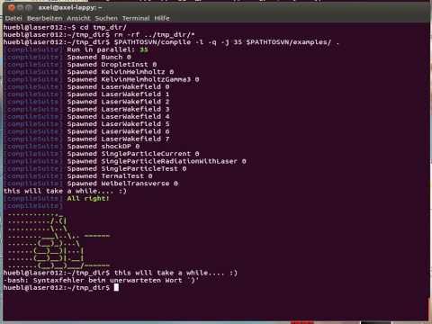 PIConGPU CompileTest
Assume
repo=<pathToYourPIConGPUgitDirectory>tmpPath=<tmpFolder>
Now run the tests with
$repo/compile -l $repo/examples/ $tmpPath
Further options are:
-q : continue on errors-j <N> : run <N> tests in parallel (note: do NOT omit the number <N>)
If you ran your test with, let’s say -l -q -j 4, and you got errors like
[compileSuite] [error] In PIC_EXTENSION_PATH:PATH=…/params/ThermalTest/cmakePreset_0: CMAKE_INSTALL_PREFIX:PATH=…/params/ThermalTest/cmakePreset_0 (…/build) make install
check the specific test’s output (in this case examples/ThermalTest with
CMake preset #0) with:
less -R $tmpPath/build/build_ThermalTest_cmakePreset_0/compile.log
Compile Tests - Single Example
Compile all CMake presets of a single example with:
$repo/compile $repo/examples/ $tmpPath
Compile Tests - Cluster Example:
Request an interactive job (to release some load from the head node)
qsub -I -q laser -lwalltime=03:00:00 -lnodes=1:ppn=64Use a non-home directory, e.g.
tmpPath=/net/cns/projects/HPL/<yourTeam>/<yourName>/tmp_tests/Compile like a boss!
<pathToYourPIConGPUgitDirectory>/compile -l -q -j 60 <pathToYourPIConGPUgitDirectory>/examples/ $tmpPathWait for the thumbs up/down :)
Repository Structure
Section author: Axel Huebl
Branches
master: the latest stable release, always tagged with a versiondev: the development branch where all features start from and are merged torelease-X.Y.Z: release candiate for versionX.Y.Zwith an upcoming release, receives updates for bug fixes and documentation such as change logs but usually no new features
Directory Structure
include/C++ header and source files
set
-Ihereprefixed with project name
lib/pre-compiled libraries
python/modules, e.g. for RT interfaces, pre* & post-processing
set
PYTHONPATHhere
etc/(runtime) configuration files
picongpu/tbgtemplates (as long as PIConGPU specific, later on toshare/tbg/)network configurations (e.g. infiniband)
score-p and vampir-trace filters
share/examples, documentation
picongpu/completions/: bash completionsexamples/: each with same structure as/
bin/core tools for the “PIConGPU framework”
set
PATHhere
docs/currently for the documentation files
might move, e.g. to
lib/picongpu/docs/and its build artifacts toshare/{doc,man}/,
Coding Guide Lines
Section author: Axel Huebl
See also
Our coding guide lines are documented in this repository.
Source Style
For contributions, an ideal patch blends in the existing coding style around it without being noticed as an addition when applied. Nevertheless, please make sure new files follow the styles linked above as strict as possible from the beginning.
clang-format-11 should be used to format the code. There are different ways to format the code.
Format All Files
To format all files in your working copy, you can run this command in bash from the root folder of PIConGPU:
find include/ share/picongpu/ share/pmacc -iname "*.def" \
-o -iname "*.h" -o -iname "*.cpp" -o -iname "*.cu" \
-o -iname "*.hpp" -o -iname "*.tpp" -o -iname "*.kernel" \
-o -iname "*.loader" -o -iname "*.param" -o -iname "*.unitless" \
| xargs clang-format-11 -i
Format Only Changes, Using Git
Instead of using the bash command above you can use Git together with ClangFormat to format your patched code only.
ClangFormat is an external tool for code formating that can be called by Git on changed files only and is part of clang tools.
Before applying this command, you must extend your local git configuration once with all file endings used in PIConGPU:
git config --local clangFormat.extensions def,h,cpp,cu,hpp,tpp,kernel,loader,param,unitless
After installing, or on a cluster loading the module(see introduction), clangFormat can be called by git on all staged files using the command:
git clangFormat
Warning
The binary for ClangFormat is called clang-format on some operating systems. If clangFormat is not recognized, try clang-format instead, in addition please check that clang-format –version returns version 11.X.X in this case.
The Typical workflow using git clangFormat is the following,
make your patch
stage the changed files in git
git add <files you changed>/ -A
format them according to guidelines
git clangFormat
stage the now changed(formated) files again
git add <files you changed>
commit changed files
git commit -m <commit message>
Please be aware that un-staged changes will not be formatted. Formatting all changes of the previous commit can be achieved by executing the command git clang-format-11 HEAD~1.
License Header
Please add the according license header snippet to your new files:
for PIConGPU (GPLv3+):
src/tools/bin/addLicense <FileName>for libraries (LGPLv3+ & GPLv3+):
export PROJECT_NAME=PMacc && src/tools/bin/addLicense <FileName>delete other headers:
src/tools/bin/deleteHeadComment <FileName>add license to all
.hppfiles within a directory (recursive):export PROJECT_NAME=PIConGPU && src/tools/bin/findAndDo <PATH> "*.hpp" src/tools/bin/addLicensethe default project name is
PIConGPU(case sensitive!) and add the GPLv3+ only
Files in the directory thirdParty/ are only imported from remote repositories.
If you want to improve them, submit your pull requests there and open an issue for our maintainers to update to a new version of the according software.
Sphinx
Section author: Axel Huebl, Marco Garten
In the following section we explain how to contribute to this documentation.
If you are reading the HTML version on http://picongpu.readthedocs.io and want to improve or correct existing pages, check the “Edit on GitHub” link on the right upper corner of each document.
Alternatively, go to docs/source in our source code and follow the directory structure of reStructuredText (.rst) files there.
For intrusive changes, like structural changes to chapters, please open an issue to discuss them beforehand.
Build Locally
This document is build based on free open-source software, namely Sphinx, Doxygen (C++ APIs as XML) and Breathe (to include doxygen XML in Sphinx). A web-version is hosted on ReadTheDocs.
The following requirements need to be installed (once) to build our documentation successfully:
cd docs/
# doxygen is not shipped via pip, install it externally,
# from the homepage, your package manager, conda, etc.
# example:
sudo apt-get install doxygen
# python tools & style theme
pip install -r requirements.txt # --user
In order to not break any of your existing Python configurations, you can also create a new environment that you only use for building the documentation. Since it is possible to install doxygen with conda, the following demonstrates this.
cd docs/
# create a bare conda environment containing just all the requirements
# for building the picongpu documentation
# note: also installs doxygen inside this environment
conda env create --file picongpu-docs-env.yml
# start up the environment as suggested during its creation e.g.
conda activate picongpu-docs-env
# or
source activate picongpu-docs-env
With all documentation-related software successfully installed, just run the following commands to build your docs locally. Please check your documentation build is successful and renders as you expected before opening a pull request!
# skip this if you are still in docs/
cd docs/
# parse the C++ API documentation,
# enjoy the doxygen warnings!
doxygen
# render the `.rst` files and replace their macros within
# enjoy the breathe errors on things it does not understand from doxygen :)
make html
# open it, e.g. with firefox :)
firefox build/html/index.html
# now again for the pdf :)
make latexpdf
# open it, e.g. with okular
build/latex/PIConGPU.pdf
Doxygen
Section author: Axel Huebl
An online version of our Doxygen build can be found at
http://computationalradiationphysics.github.io/picongpu
We regularly update it via
git checkout gh-pages
# optional argument: branch or tag name
./update.sh
git commit -a
git push
This section explains what is done when this script is run to build it manually.
Requirements
First, install Doxygen and its dependencies for graph generation.
# install requirements (Debian/Ubuntu)
sudo apt-get install doxygen graphviz
# enable HTML output in our Doxyfile
sed -i 's/GENERATE_HTML.*=.*NO/GENERATE_HTML = YES/' docs/Doxyfile
Build
Now run the following commands to build the Doxygen HTML documentation locally.
cd docs/
# build the doxygen HTML documentation
doxygen
# open the generated HTML pages, e.g. with firefox
firefox html/index.html
Clang Tools
Section author: Axel Huebl
We are currently integrating support for Clang Tools [ClangTools] such as clang-tidy and clang-format.
Clang Tools are fantastic for static source code analysis, e.g. to find defects, automate style formatting or modernize code.
Install
At least LLVM/Clang 3.9 or newer is required. On Debian/Ubuntu, install them via:
sudo apt-get install clang-tidy-3.9
Usage
Currently, those tools work only with CPU backends of PIConGPU. For example, enable the OpenMP backend via:
# in an example
mkdir .build
cd build
pic-configure -c"-DALPAKA_ACC_CPU_B_OMP2_T_SEQ_ENABLE=ON" ..
We try to auto-detect clang-tidy.
If that fails, you can set a manual hint to an adequate version via -DCLANG_TIDY_BIN in CMake:
pic-configure -c"-DALPAKA_ACC_CPU_B_OMP2_T_SEQ_ENABLE=ON -DCLANG_TIDY_BIN=$(which clang-tidy-3.9)" ..
If a proper version of clang-tidy is found, we add a new clang-tidy build target:
# enable verbose output to see all warnings and errors
make VERBOSE=true clang-tidy
- ClangTools
Online (2017), https://clang.llvm.org/docs/ClangTools.html
Extending PIConGPU
Section author: Sergei Bastrakov
Note
A number of places in .param files allow providing user-defined functors. The processing logic can largely be customized on that level, without modifying the source code. Such an external way is recommended when applicable. This section covers the case of extending the internal implementation.
General Simulation Loop Structure
A PIConGPU simulation effectively boils down to performing initialization and then executing a simulation loop. The simulation loop iterates over the requested number of time steps. For each time step, first all enabled plugins are called. Then all core computational stages are executed. Details of creating a new plugin or a new stage are presented below.
Adding a Plugin
PIConGPU plugins can perform computations or output, and often do both. Since all plugins are called at iteration start, they normally implement operations that are independent of the place in the computational loop. For operations requiring a specific ordering, please refer to the next section.
To add a new plugin, make a new file or subdirectory inside include/picongpu/plugins.
Each plugin class must inherit our base class ISimulationPlugin.
In turn, it largely uses its own base class pmacc::ISimulationPlugin.
These classes define the interface of all PIConGPU plugins.
The methods that most plugins want to override are:
pluginRegisterHelp()adds command-line options for the plugin. In case a plugin introduces some new compile-time parameters, they are normally put to a new.paramfile.pluginGetName()sets a text name for the plugin, used to report errors currently.pluginLoad()initializes internal data of the plugin after the command-line arguments are submitted. Note that a constructor of the plugin class would be called before that and so often cannot do a full initialization. Is called once upon simulation start.pluginUnload()finalizes internal data if necessary, is called once at the end of the simulation.setMappingDescription()is used to pass simulation data to be used in kernelsnotify()runs the plugin for the given time iteration. This method implements the computational logic of the plugin. It often involves calling an internal algorithm or writing an own kernel. Those are described in the following sections.checkpoint()saves plugin internal data for checkpointing if necessaryrestart()loads the internal data from a checkpoint (necessary ifcheckpoint()writes some data)
Most plugins are run with a certain period in time steps.
In this case, Environment<>::get().PluginConnector().setNotificationPeriod(this, notifyPeriod) can be used inside pluginLoad() to set this period.
Then notify() will only be called for the active time steps.
For plugins (and most PIConGPU code) dealing with particles, it is common to template-parametrize based on species.
Such plugins should use base class plugins::multi::IInstance.
There is also a helper class plugins::multi::IHelp for command-line parameters prefixed for species.
To match a plugin to applicable species, partially specialize trait particles::traits::SpeciesEligibleForSolver.
Regardless of the base class used, the new plugin class must be instantiated at picongpu::PluginController and the new headers included there.
In case the plugin is conditionally available (e.g. requires an optional dependency), guards must also be placed there, around the include and instantiation.
When adding a plugin, do not forget to extend the documentation with plugin description and parameters.
At least, extend the list of plugins and command-line parameters (the latter via TBG_macros.cfg).
Other welcome additions for a new plugin include a dedicated documentation, a new example demonstrating usage in a realistic scenario, and a Python postprocessing script.
Adding a Simulation Stage
The currently executed simulation stages and their order are defined inside Simulation::runOneStep().
All stage classes are in namespace picongpu::simulation::stage and their implementations are located in respective directory.
The existing stages share compatible interface and thus follow a pseudo-concept, not formally defined currently.
The interface is also compatible to functors passed to InitPipeline and IterationStartPipeline.
Note that stage classes are just wrappers around the internal implementations.
Their purpose is to offer a high-level view of the steps and data dependencies in the computational loop, and add command-line parameters if necessary.
To add a new simulation stage:
create a new
.hppfile inpicongpu/simulation/stage.write your stage functor class following the interface of other stage functors.
if needed (e.g. for command-line parameters or static data) store an instance of it as a member of
Simulationclass.add a call to it inside
Simulation::runOneStep().
As mentioned above, a simulation stage should merely be calling an actual implementation located at an appropriate place inside PIConGPU or pmacc.
When possible, it is recommended to use existing generic algorithms like particles::Manipulate<> or FieldTmp::computeValue().
Otherwise, one often has to implement an own kernel.
Writing a Kernel
Computational kernels are written using library cupla which is a layer on top of library alpaka.
Most kernel functors are templates parametrized with the number of threads per block, often called numWorkers.
Kernel invocations are wrapped into a helper macro PMACC_KERNEL.
A vast majority of PIConGPU kernels operate on two levels of parallelism: between supercells and inside each supercell. This parallel pattern is covered by the mapper concept.
-
template<uint32_t
T_areaType, template<unsigned, typename> classT_MappingDescription, unsignedT_dim, typenameT_SupercellSize>
classMapperConcept: public T_MappingDescription<T_dim, T_SupercellSize>¶ Concept for mapper from block indices to supercells in the given area for alpaka kernels.
The mapping covers the case of supercell-level parallelism between alpaka blocks. The supercells can be processed concurrently in any order. This class is not used directly, but defines a concept for such mappers.
Mapper provides a 1:1 mapping from supercells in the area to alpaka blocks. (Since it is 1:1, the mapping is invertible, but only this direction is provided.) Dimensionality of the area indices and block indices is the same. A kernel must be launched with exactly getGridDim() blocks. Each block must process a single supercell with index getSuperCellIndex(blockIndex). Implementation is optimized for the standard areas in AreaType.
In-block parallelism is independent of this mapping and is done by a kernel. Naturally, this parallelism should also define block size, again independent of this mapping.
This pattern is used in most kernels in particle-mesh codes. Two most common parallel patterns are:
for particle or particle-grid operations: alpaka block per supercell with this mapping, thread-level parallelism between particles of a frame
for grid operations: alpaka block per supercell with this mapping, thread-level parallelism between cells of a supercell
- Template Parameters
T_areaType: parameter describing area to be mapped (depends on mapper type)T_MappingDescription: mapping description type, base class for MapperConceptT_dim: dimensionality of area and block indicesT_SupercellSize: compile-time supercell size
For this parallel pattern, a mapper object provides the number of blocks to use for a kernel. On the device side, the object provides a mapping between alpaka blocks and supercells to be processed. Parallelism for threads between blocks is done inside the kernel. It is often over cells in a supercell or particles in a frame using lockstep programming.
A kernel often takes one or several data boxes from the host side. The data boxes allow array-like access to data. A more detailed description of boxes and other widely used classes is given in the following sections.
Important PIConGPU Classes
This is very, very small selection of classes of interest to get you started.
Simulation
-
class
Simulation: public pmacc::SimulationHelper<simDim>¶ Global simulation controller class.
Initialises simulation data and defines the simulation steps for each iteration.
- Template Parameters
DIM: the dimension (2-3) for the simulation
Public Functions
-
Simulation()¶ Constructor.
-
void
pluginRegisterHelp(po::options_description &desc)¶ Register command line parameters for this plugin.
Parameters are parsed and set prior to plugin load.
- Parameters
desc: boost::program_options description
-
std::string
pluginGetName() const¶ Return the name of this plugin for status messages.
- Return
plugin name
-
void
pluginLoad()
-
void
pluginUnload()
-
void
notify(uint32_t currentStep)¶ Notification callback.
For example Plugins can set their requested notification frequency at the PluginConnector
- Parameters
currentStep: current simulation iteration step
-
void
init()¶ Initialize simulation.
Does hardware selections/reservations, memory allocations and initializes data structures as empty.
-
uint32_t
fillSimulation()¶ Fills simulation with initial data after init()
- Return
returns the first step of the simulation (can be >0 for, e.g., restarts from checkpoints)
-
void
runOneStep(uint32_t currentStep)¶ Run one simulation step.
- Parameters
currentStep: iteration number of the current step
-
void
movingWindowCheck(uint32_t currentStep)¶ Check if moving window work must do.
If no moving window is needed the implementation of this function can be empty
- Parameters
currentStep: simulation step
-
void
resetAll(uint32_t currentStep)¶ Reset the simulation to a state such as it was after init() but for a specific time step.
Can be used to call fillSimulation() again.
-
void
slide(uint32_t currentStep)
-
virtual void
setInitController(IInitPlugin *initController)
-
MappingDesc *
getMappingDescription()
FieldE
-
class
FieldE: public picongpu::fields::EMFieldBase<FieldE>¶ Representation of the electric field.
Stores field values on host and device and provides data synchronization between them.
Implements interfaces defined by SimulationFieldHelper< MappingDesc > and ISimulationData.
FieldB
-
class
FieldB: public picongpu::fields::EMFieldBase<FieldB>¶ Representation of the magnetic field.
Stores field values on host and device and provides data synchronization between them.
Implements interfaces defined by SimulationFieldHelper< MappingDesc > and ISimulationData.
FieldJ
-
class
FieldJ: public pmacc::SimulationFieldHelper<MappingDesc>, public pmacc::ISimulationData¶ Representation of the current density field.
Stores field values on host and device and provides data synchronization between them.
Implements interfaces defined by SimulationFieldHelper< MappingDesc > and ISimulationData.
FieldTmp
-
class
FieldTmp: public pmacc::SimulationFieldHelper<MappingDesc>, public pmacc::ISimulationData¶ Representation of the temporary scalar field for plugins and temporary particle data mapped to grid (charge density, energy density, etc.)
Stores field values on host and device and provides data synchronization between them.
Implements interfaces defined by SimulationFieldHelper< MappingDesc > and ISimulationData.
Particles
-
template<typename
T_Name, typenameT_Flags, typenameT_Attributes>
classParticles: public pmacc::ParticlesBase<ParticleDescription<T_Name, SuperCellSize, T_Attributes, T_Flags, bmpl::if_<bmpl::contains<T_Flags, GetKeyFromAlias<T_Flags, boundaryCondition<>>::type>, pmacc::traits::Resolve<GetKeyFromAlias<T_Flags, boundaryCondition<>>::type>::type, pmacc::HandleGuardRegion<pmacc::particles::policies::ExchangeParticles, pmacc::particles::policies::DoNothing>>::type>, MappingDesc, DeviceHeap>, public pmacc::ISimulationData¶ particle species
- Template Parameters
T_Name: name of the species [type boost::mpl::string]T_Attributes: sequence with attributes [type boost::mpl forward sequence]T_Flags: sequence with flags e.g. solver [type boost::mpl forward sequence]
Public Types
-
template<>
usingSpeciesParticleDescription= pmacc::ParticleDescription<T_Name, SuperCellSize, T_Attributes, T_Flags, typename bmpl::if_<bmpl::contains<T_Flags, typename GetKeyFromAlias<T_Flags, boundaryCondition<>>::type>, typename pmacc::traits::Resolve<typename GetKeyFromAlias<T_Flags, boundaryCondition<>>::type>::type, pmacc::HandleGuardRegion<pmacc::particles::policies::ExchangeParticles, pmacc::particles::policies::DoNothing>>::type>
-
template<>
usingParticlesBaseType= ParticlesBase<SpeciesParticleDescription, picongpu::MappingDesc, DeviceHeap>
-
template<>
usingFrameType= typename ParticlesBaseType::FrameType
-
template<>
usingFrameTypeBorder= typename ParticlesBaseType::FrameTypeBorder
-
template<>
usingParticlesBoxType= typename ParticlesBaseType::ParticlesBoxType
Public Functions
-
void
createParticleBuffer()
-
void
update(uint32_t const currentStep)¶ Push all particles.
-
template<typename
T_MapperFactory>
voidshiftBetweenSupercells(T_MapperFactory const &mapperFactory, bool onlyProcessMustShiftSupercells)¶ Update the supercell storage for particles in the area according to particle attributes.
- Template Parameters
T_MapperFactory: factory type to construct a mapper that defines the area to process
- Parameters
mapperFactory: factory instanceonlyProcessMustShiftSupercells: whether to process only supercells with mustShift set to true (optimization to be used with particle pusher) or process all supercells
-
void
applyBoundary(uint32_t const currentStep)¶ Apply all boundary conditions.
-
template<typename
T_DensityFunctor, typenameT_PositionFunctor>
voidinitDensityProfile(T_DensityFunctor &densityFunctor, T_PositionFunctor &positionFunctor, const uint32_t currentStep)
-
template<typename
T_SrcName, typenameT_SrcAttributes, typenameT_SrcFlags, typenameT_ManipulateFunctor, typenameT_SrcFilterFunctor>
voiddeviceDeriveFrom(Particles<T_SrcName, T_SrcAttributes, T_SrcFlags> &src, T_ManipulateFunctor &manipulateFunctor, T_SrcFilterFunctor &srcFilterFunctor)
-
SimulationDataId
getUniqueId()¶ Return the globally unique identifier for this simulation data.
- Return
globally unique identifier
-
void
synchronize()¶ Synchronizes simulation data, meaning accessing (host side) data will return up-to-date values.
-
void
syncToDevice()¶ Synchronize data from host to device.
-
template<typename
T_Pusher>
voidpush(uint32_t const currentStep)¶ Do the particle push stage using the given pusher.
- Template Parameters
T_Pusher: non-composite pusher type
- Parameters
currentStep: current time iteration
Public Static Functions
-
static std::array<particles::boundary::Description, simDim> &
boundaryDescription()¶ Get boundary descriptions for the species.
For both sides along the same axis, both boundaries have the same description. Must not be modified outside of the ParticleBoundaries simulation stage.
This method is static as it is used by static getStringProperties().
ComputeGridValuePerFrame
-
template<class
T_ParticleShape, classT_DerivedAttribute>
classComputeGridValuePerFrame¶ Public Types
-
template<>
usingAssignmentFunction= typename T_ParticleShape::ChargeAssignment
Public Functions
-
HDINLINE
ComputeGridValuePerFrame()
-
HDINLINE float1_64 picongpu::particles::particleToGrid::ComputeGridValuePerFrame::getUnit() const return unit for this solver
- Return
solver unit
-
HINLINE std::vector< float_64 > picongpu::particles::particleToGrid::ComputeGridValuePerFrame::getUnitDimension() const return powers of the 7 base measures for this solver
characterizing the unit of the result of the solver in SI (length L, mass M, time T, electric current I, thermodynamic temperature theta, amount of substance N, luminous intensity J)
-
template<typename FrameType, typename TVecSuperCell, typename BoxTmp, typename T_Acc, typename T_AccFilter>DINLINE void picongpu::particles::particleToGrid::ComputeGridValuePerFrame::operator()(T_Acc const & acc, FrameType & frame, const int localIdx, const TVecSuperCell superCell, T_AccFilter & accFilter, BoxTmp & tmpBox)
Public Static Functions
-
HINLINE std::string picongpu::particles::particleToGrid::ComputeGridValuePerFrame::getName() return name of the this solver
- Return
name of solver
-
template<>
Important pmacc Classes
This is very, very small selection of classes of interest to get you started.
Note
Please help adding more Doxygen doc strings to the classes described below. As an example, here is a listing of possible extensive docs that new developers find are missing: https://github.com/ComputationalRadiationPhysics/picongpu/issues/776
Environment
-
template<uint32_t
T_dim>
classEnvironment: public pmacc::detail::Environment¶ Global Environment singleton for PMacc.
Public Functions
-
void
enableMpiDirect()
-
bool
isMpiDirectEnabled() const
-
pmacc::GridController<T_dim> &
GridController()¶ get the singleton GridController
- Return
instance of GridController
-
void
initDevices(DataSpace<T_dim> devices, DataSpace<T_dim> periodic)¶ create and initialize the environment of PMacc
Usage of MPI or device(accelerator) function calls before this method are not allowed.
- Parameters
devices: number of devices per simulation dimensionperiodic: periodicity each simulation dimension (0 == not periodic, 1 == periodic)
-
void
initGrids(DataSpace<T_dim> globalDomainSize, DataSpace<T_dim> localDomainSize, DataSpace<T_dim> localDomainOffset)¶ initialize the computing domain information of PMacc
- Parameters
globalDomainSize: size of the global simulation domain [cells]localDomainSize: size of the local simulation domain [cells]localDomainOffset: local domain offset [cells]
-
Environment(const Environment&)
-
Environment &
operator=(const Environment&)
Public Static Functions
-
static Environment<T_dim> &
get()¶ get the singleton Environment< DIM >
- Return
instance of Environment<DIM >
-
void
DataConnector
-
class
DataConnector¶ Singleton class which collects and shares simulation data.
All members are kept as shared pointers, which allows their factories to be destroyed after sharing ownership with our DataConnector.
Public Functions
-
bool
hasId(SimulationDataId id)¶ Returns if data with identifier id is shared.
- Return
if dataset with id is registered
- Parameters
id: id of the Dataset to query
-
void
initialise(AbstractInitialiser &initialiser, uint32_t currentStep)¶ Initialises all Datasets using initialiser.
After initialising, the Datasets will be invalid.
- Parameters
initialiser: class used for initialising DatasetscurrentStep: current simulation step
Register a new Dataset and share its ownership.
If a Dataset with the same id already exists, a runtime_error is thrown. (Check with DataConnector::hasId when necessary.)
- Parameters
data: simulation data to share ownership
-
void
consume(std::unique_ptr<ISimulationData> data)¶ Register a new Dataset and transfer its ownership.
If a Dataset with the same id already exists, a runtime_error is thrown. (Check with DataConnector::hasId when necessary.) The only difference from share() is transfer of ownership.
- Parameters
data: simulation data to transfer ownership
-
void
deregister(SimulationDataId id)¶ End sharing a dataset with identifier id.
- Parameters
id: id of the dataset to remove
-
void
clean()¶ Unshare all associated datasets.
Returns shared pointer to managed data.
Reference to data in Dataset with identifier id and type TYPE is returned. If the Dataset status in invalid, it is automatically synchronized. Increments the reference counter to the dataset specified by id.
- Return
returns a reference to the data of type TYPE
- Template Parameters
TYPE: if of the data to load
- Parameters
id: id of the Dataset to load fromnoSync: indicates that no synchronization should be performed, regardless of dataset status
Friends
-
friend
pmacc::DataConnector::detail::Environment
-
bool
DataSpace
-
template<unsigned
T_Dim>
classDataSpace: public pmacc::math::Vector<int, T_Dim>¶ A T_Dim-dimensional data space.
DataSpace describes a T_Dim-dimensional data space with a specific size for each dimension. It only describes the space and does not hold any actual data.
- Template Parameters
T_Dim: dimension (1-3) of the dataspace
Public Types
-
template<>
usingBaseType= math::Vector<int, T_Dim>
Public Functions
-
HDINLINE
DataSpace()¶ default constructor.
Sets size of all dimensions to 0.
-
constexpr HDINLINE DataSpace& pmacc::DataSpace::operator=(const DataSpace &)
-
HDINLINE
DataSpace(cupla::dim3 value)¶ constructor.
Sets size of all dimensions from cuda dim3.
-
HDINLINE
DataSpace(cupla::uint3 value)¶ constructor.
Sets size of all dimensions from cupla uint3 (e.g. cupla::threadIdx(acc)/cupla::blockIdx(acc))
-
HDINLINE
DataSpace(int x)¶ Constructor for DIM1-dimensional DataSpace.
- Parameters
x: size of first dimension
-
HDINLINE
DataSpace(int x, int y)¶ Constructor for DIM2-dimensional DataSpace.
- Parameters
x: size of first dimensiony: size of second dimension
-
HDINLINE
DataSpace(int x, int y, int z)¶ Constructor for DIM3-dimensional DataSpace.
- Parameters
x: size of first dimensiony: size of second dimensionz: size of third dimension
-
HDINLINE
DataSpace(const BaseType &vec)
-
HDINLINE
DataSpace(const math::Size_t<T_Dim> &vec)
-
HDINLINE int pmacc::DataSpace::getDim() const Returns number of dimensions (T_Dim) of this DataSpace.
- Return
number of dimensions
-
HINLINE bool pmacc::DataSpace::isOneDimensionGreaterThan(const DataSpace < T_Dim > & other) const Evaluates if one dimension is greater than the respective dimension of other.
- Return
true if one dimension is greater, false otherwise
- Parameters
other: DataSpace to compare with
-
HDINLINE
operator math::Size_t<T_Dim>() const
-
HDINLINE
operator cupla::dim3() const
Public Static Functions
Public Static Attributes
-
constexpr int
Dim= T_Dim
Vector
Warning
doxygenclass: Cannot find class “pmacc::math::Vector” in doxygen xml output for project “PIConGPU” from directory: ../xml
SuperCell
-
template<class
T_FrameType>
classSuperCell¶ Public Functions
-
HDINLINE
SuperCell()
-
HDINLINE T_FrameType* pmacc::SuperCell::FirstFramePtr()
-
HDINLINE T_FrameType* pmacc::SuperCell::LastFramePtr()
-
HDINLINE T_FrameType const* pmacc::SuperCell::FirstFramePtr() const
-
HDINLINE T_FrameType const* pmacc::SuperCell::LastFramePtr() const
-
HDINLINE bool pmacc::SuperCell::mustShift() const
-
HDINLINE void pmacc::SuperCell::setMustShift(bool const value)
-
HDINLINE uint32_t pmacc::SuperCell::getSizeLastFrame() const
-
HDINLINE uint32_t pmacc::SuperCell::getNumParticles() const
-
HDINLINE void pmacc::SuperCell::setNumParticles(uint32_t const size)
-
PMACC_ALIGN(firstFramePtr, T_FrameType *)
-
PMACC_ALIGN(lastFramePtr, T_FrameType *)
-
HDINLINE
GridBuffer
-
template<class
TYPE, unsignedDIM, classBORDERTYPE= TYPE>
classGridBuffer: public pmacc::HostDeviceBuffer<TYPE, DIM>¶ GridBuffer represents a DIM-dimensional buffer which exists on the host as well as on the device.
GridBuffer combines a HostBuffer and a DeviceBuffer with equal sizes. Additionally, it allows sending data from and receiving data to these buffers. Buffers consist of core data which may be surrounded by border data.
- Template Parameters
TYPE: datatype for internal Host- and DeviceBufferDIM: dimension of the buffersBORDERTYPE: optional type for border data in the buffers. TYPE is used by default.
Public Types
-
template<>
usingDataBoxType= typename Parent::DataBoxType
Public Functions
-
GridBuffer(const GridLayout<DIM> &gridLayout, bool sizeOnDevice = false)¶ Constructor.
- Parameters
gridLayout: layout of the buffers, including border-cellssizeOnDevice: if true, size information exists on device, too.
-
GridBuffer(const DataSpace<DIM> &dataSpace, bool sizeOnDevice = false)¶ Constructor.
- Parameters
dataSpace: DataSpace representing buffer size without border-cellssizeOnDevice: if true, internal buffers must store their size additionally on the device (as we keep this information coherent with the host, it influences performance on host-device copies, but some algorithms on the device might need to know the size of the buffer)
-
GridBuffer(DeviceBuffer<TYPE, DIM> &otherDeviceBuffer, const GridLayout<DIM> &gridLayout, bool sizeOnDevice = false)¶ Constructor.
- Parameters
otherDeviceBuffer: DeviceBuffer which should be used instead of creating own DeviceBuffergridLayout: layout of the buffers, including border-cellssizeOnDevice: if true, internal buffers must store their size additionally on the device (as we keep this information coherent with the host, it influences performance on host-device copies, but some algorithms on the device might need to know the size of the buffer)
-
GridBuffer(HostBuffer<TYPE, DIM> &otherHostBuffer, const DataSpace<DIM> &offsetHost, DeviceBuffer<TYPE, DIM> &otherDeviceBuffer, const DataSpace<DIM> &offsetDevice, const GridLayout<DIM> &gridLayout, bool sizeOnDevice = false)
-
void
addExchange(uint32_t dataPlace, const Mask &receive, DataSpace<DIM> guardingCells, uint32_t communicationTag, bool sizeOnDeviceSend, bool sizeOnDeviceReceive)¶ Add Exchange in GridBuffer memory space.
An Exchange is added to this GridBuffer. The exchange buffers use the same memory as this GridBuffer.
- Parameters
dataPlace: place where received data is stored [GUARD | BORDER] if dataPlace=GUARD than copy other BORDER to my GUARD if dataPlace=BORDER than copy other GUARD to my BORDERreceive: a Mask which describes the directions for the exchangeguardingCells: number of guarding cells in each dimensioncommunicationTag: unique tag/id for communication has to be the same when this method is called multiple times for the same object (with non-overlapping masks)sizeOnDeviceSend: if true, internal send buffers must store their size additionally on the device (as we keep this information coherent with the host, it influences performance on host-device copies, but some algorithms on the device might need to know the size of the buffer)sizeOnDeviceReceive: if true, internal receive buffers must store their size additionally on the device
-
void
addExchange(uint32_t dataPlace, const Mask &receive, DataSpace<DIM> guardingCells, uint32_t communicationTag, bool sizeOnDevice = false)¶ Add Exchange in GridBuffer memory space.
An Exchange is added to this GridBuffer. The exchange buffers use the same memory as this GridBuffer.
- Parameters
dataPlace: place where received data is stored [GUARD | BORDER] if dataPlace=GUARD than copy other BORDER to my GUARD if dataPlace=BORDER than copy other GUARD to my BORDERreceive: a Mask which describes the directions for the exchangeguardingCells: number of guarding cells in each dimensioncommunicationTag: unique tag/id for communicationsizeOnDevice: if true, internal buffers must store their size additionally on the device (as we keep this information coherent with the host, it influences performance on host-device copies, but some algorithms on the device might need to know the size of the buffer)
-
void
addExchangeBuffer(const Mask &receive, const DataSpace<DIM> &dataSpace, uint32_t communicationTag, bool sizeOnDeviceSend, bool sizeOnDeviceReceive)¶ Add Exchange in dedicated memory space.
An Exchange is added to this GridBuffer. The exchange buffers use the their own memory instead of using the GridBuffer’s memory space.
- Parameters
receive: a Mask which describes the directions for the exchangedataSpace: size of the newly created exchange buffer in each dimensioncommunicationTag: unique tag/id for communicationsizeOnDeviceSend: if true, internal send buffers must store their size additionally on the device (as we keep this information coherent with the host, it influences performance on host-device copies, but some algorithms on the device might need to know the size of the buffer)sizeOnDeviceReceive: if true, internal receive buffers must store their size additionally on the device
-
void
addExchangeBuffer(const Mask &receive, const DataSpace<DIM> &dataSpace, uint32_t communicationTag, bool sizeOnDevice = false)¶ Add Exchange in dedicated memory space.
An Exchange is added to this GridBuffer. The exchange buffers use the their own memory instead of using the GridBuffer’s memory space.
- Parameters
receive: a Mask which describes the directions for the exchangedataSpace: size of the newly created exchange buffer in each dimensioncommunicationTag: unique tag/id for communicationsizeOnDevice: if true, internal buffers must store their size additionally on the device (as we keep this information coherent with the host, it influences performance on host-device copies, but some algorithms on the device might need to know the size of the buffer)
-
bool
hasSendExchange(uint32_t ex) const¶ Returns whether this GridBuffer has an Exchange for sending in ex direction.
- Return
true if send exchanges with ex direction exist, otherwise false
- Parameters
ex: exchange direction to query
-
bool
hasReceiveExchange(uint32_t ex) const¶ Returns whether this GridBuffer has an Exchange for receiving from ex direction.
- Return
true if receive exchanges with ex direction exist, otherwise false
- Parameters
ex: exchange direction to query
-
Exchange<BORDERTYPE, DIM> &
getSendExchange(uint32_t ex) const¶ Returns the Exchange for sending data in ex direction.
Returns an Exchange which for sending data from this GridBuffer in the direction described by ex.
- Return
the Exchange for sending data
- Parameters
ex: the direction to query
-
Exchange<BORDERTYPE, DIM> &
getReceiveExchange(uint32_t ex) const¶ Returns the Exchange for receiving data from ex direction.
Returns an Exchange which for receiving data to this GridBuffer from the direction described by ex.
- Return
the Exchange for receiving data
- Parameters
ex: the direction to query
-
Mask
getSendMask() const¶ Returns the Mask describing send exchanges.
- Return
Mask for send exchanges
-
Mask
getReceiveMask() const¶ Returns the Mask describing receive exchanges.
- Return
Mask for receive exchanges
-
EventTask
communication()¶ Starts sync data from own device buffer to neighbor device buffer.
Asynchronously starts synchronization data from internal DeviceBuffer using added Exchange buffers. This operation runs sequential to other code but intern asynchronous
-
EventTask
asyncCommunication(EventTask serialEvent)¶ Starts sync data from own device buffer to neighbor device buffer.
Asynchronously starts synchronization data from internal DeviceBuffer using added Exchange buffers.
-
EventTask
asyncSend(EventTask serialEvent, uint32_t sendEx)
-
EventTask
asyncReceive(EventTask serialEvent, uint32_t recvEx)
-
GridLayout<DIM>
getGridLayout()¶ Returns the GridLayout describing this GridBuffer.
- Return
the layout of this buffer
Protected Attributes
-
bool
hasOneExchange
-
uint32_t
lastUsedCommunicationTag
-
GridLayout<DIM>
gridLayout
-
Mask
sendMask
-
Mask
receiveMask
-
template<>
std::unique_ptr<ExchangeIntern<BORDERTYPE, DIM>>sendExchanges[27]
-
template<>
std::unique_ptr<ExchangeIntern<BORDERTYPE, DIM>>receiveExchanges[27]
-
template<>
EventTaskreceiveEvents[27]
-
template<>
EventTasksendEvents[27]
-
uint32_t
maxExchange
SimulationFieldHelper
-
template<class
CellDescription>
classSimulationFieldHelper¶ Public Types
-
template<>
usingMappingDesc= CellDescription
Public Functions
-
SimulationFieldHelper(CellDescription description)
-
virtual
~SimulationFieldHelper()
-
virtual void
reset(uint32_t currentStep) = 0¶ Reset is as well used for init.
-
virtual void
syncToDevice() = 0¶ Synchronize data from host to device.
-
CellDescription
getCellDescription() const
Protected Attributes
-
CellDescription
cellDescription
-
template<>
ParticlesBase
-
template<typename
T_ParticleDescription, classT_MappingDesc, typenameT_DeviceHeap>
classParticlesBase: public pmacc::SimulationFieldHelper<T_MappingDesc>¶ Public Types
-
enum [anonymous]
Values:
-
Dim= MappingDesc::Dim
-
TileSize= math::CT::volume<typename MappingDesc::SuperCellSize>::type::value
-
-
template<>
usingBufferType= ParticlesBuffer<ParticleDescription, typename MappingDesc::SuperCellSize, T_DeviceHeap, MappingDesc::Dim>
-
template<>
usingFrameType= typename BufferType::FrameType
-
template<>
usingFrameTypeBorder= typename BufferType::FrameTypeBorder
-
template<>
usingParticlesBoxType= typename BufferType::ParticlesBoxType
-
template<>
usingHandleGuardRegion= typename ParticleDescription::HandleGuardRegion
-
template<>
usingSimulationDataTag= ParticlesTag
Public Functions
-
template<typename
T_MapperFactory>
voidfillGaps(T_MapperFactory const &mapperFactory)¶ Fill gaps in an area defined by a mapper factory.
- Template Parameters
T_MapperFactory: factory type to construct a mapper that defines the area to process
- Parameters
mapperFactory: factory instance
-
void
fillAllGaps()
-
void
fillBorderGaps()
-
void
deleteGuardParticles(uint32_t exchangeType)
-
template<uint32_t
T_area>
voiddeleteParticlesInArea()
-
void
copyGuardToExchange(uint32_t exchangeType)¶ copy guard particles to intermediate exchange buffer
Copy all particles from the guard of a direction to the device exchange buffer.
- Warning
This method resets the number of particles in the processed supercells even if there are particles left in the supercell and does not guarantee that the last frame is contiguous filled. Call fillAllGaps afterwards if you need a valid number of particles and a contiguously filled last frame.
-
void
insertParticles(uint32_t exchangeType)
-
ParticlesBoxType
getDeviceParticlesBox()
-
ParticlesBoxType
getHostParticlesBox(const int64_t memoryOffset)
-
BufferType &
getParticlesBuffer()
-
void
reset(uint32_t currentStep)¶ Reset is as well used for init.
Protected Functions
-
~ParticlesBase()
-
template<uint32_t
T_area>
voidshiftParticles(bool onlyProcessMustShiftSupercells)¶ Shift all particles in an area defined by a mapper factory.
The factory type must be such that StrideMapperFactory<T_MapperFactory, stride> is specialized
- Parameters
onlyProcessMustShiftSupercells: whether to process only supercells with mustShift set to true (optimization to be used with particle pusher) or process all supercells
-
template<typename
T_MapperFactory>
voidshiftParticles(T_MapperFactory const &mapperFactory, bool onlyProcessMustShiftSupercells)¶ Shift all particles in the area defined by the given factory.
Note that the area itself is not strided, but the factory must produce stride mappers for the area.
- Template Parameters
T_strideMapperFactory: factory type to construct a stride mapper, resulting mapper must have stride of at least 3, adheres to the MapperFactory concept
- Parameters
mapperFactory: factory instanceonlyProcessMustShiftSupercells: whether to process only supercells with mustShift set to true (optimization to be used with particle pusher) or process all supercells
Protected Attributes
-
BufferType *
particlesBuffer
-
enum [anonymous]
ParticleDescription
-
template<typename
T_Name, typenameT_SuperCellSize, typenameT_ValueTypeSeq, typenameT_Flags= bmpl::vector0<>, typenameT_HandleGuardRegion= HandleGuardRegion<particles::policies::ExchangeParticles, particles::policies::DeleteParticles>, typenameT_MethodsList= bmpl::vector0<>, typenameT_FrameExtensionList= bmpl::vector0<>>
structParticleDescription¶ ParticleDescription defines attributes, methods and flags of a particle.
This class holds no runtime data. The class holds information about the name, attributes, flags and methods of a particle.
- Template Parameters
T_Name: name of described particle (e.g. electron, ion) type must be a boost::mpl::stringT_SuperCellSize: compile time size of a super cellT_ValueTypeSeq: sequence or single type with value_identifierT_Flags: sequence or single type with identifier to add flags on a frameT_MethodsList: sequence or single class with particle methods (e.g. calculate mass, gamma, …) (e.g. useSolverXY, calcRadiation, …)T_FrameExtensionList: sequence or single class with frame extensionsextension must be an unary template class that supports bmpl::apply1<>
type of the final frame is applied to each extension class (this allows pointers and references to a frame itself)
the final frame that uses ParticleDescription inherits from all extension classes
Public Types
-
template<>
usingName= T_Name
-
template<>
usingSuperCellSize= T_SuperCellSize
-
template<>
usingValueTypeSeq= typename ToSeq<T_ValueTypeSeq>::type
-
template<>
usingFlagsList= typename ToSeq<T_Flags>::type
-
template<>
usingHandleGuardRegion= T_HandleGuardRegion
-
template<>
usingMethodsList= typename ToSeq<T_MethodsList>::type
-
template<>
usingFrameExtensionList= typename ToSeq<T_FrameExtensionList>::type
-
template<>
usingThisType= ParticleDescription<Name, SuperCellSize, ValueTypeSeq, FlagsList, HandleGuardRegion, MethodsList, FrameExtensionList>
ParticleBox
Warning
doxygenstruct: Cannot find class “pmacc::ParticlesBox” in doxygen xml output for project “PIConGPU” from directory: ../xml
Frame
-
template<typename
T_CreatePairOperator, typenameT_ParticleDescription>
structFrame: public pmacc::InheritLinearly<T_ParticleDescription::MethodsList>, protected pmacc::math::MapTuple<SeqToMap<T_ParticleDescription::ValueTypeSeq, T_CreatePairOperator>::type, pmath::AlignedData>, public pmacc::InheritLinearly<OperateOnSeq<T_ParticleDescription::FrameExtensionList, bmpl::apply1<bmpl::_1, Frame<T_CreatePairOperator, T_ParticleDescription>>>::type>¶ Frame is a storage for arbitrary number >0 of Particles with attributes.
- See
MapTupel
- Template Parameters
T_CreatePairOperator: unary template operator to create a boost pair from single type ( pair<name,dataType> )
- Template Parameters
T_ValueTypeSeq: sequence with value_identifierT_MethodsList: sequence of classes with particle methods (e.g. calculate mass, gamma, …)T_Flags: sequence with identifiers to add flags on a frame (e.g. useSolverXY, calcRadiation, …)
Public Types
-
template<>
usingParticleDescription= T_ParticleDescription
-
template<>
usingName= typename ParticleDescription::Name
-
template<>
usingSuperCellSize= typename ParticleDescription::SuperCellSize
-
template<>
usingValueTypeSeq= typename ParticleDescription::ValueTypeSeq
-
template<>
usingMethodsList= typename ParticleDescription::MethodsList
-
template<>
usingFlagList= typename ParticleDescription::FlagsList
-
template<>
usingFrameExtensionList= typename ParticleDescription::FrameExtensionList
-
template<>
usingThisType= Frame<T_CreatePairOperator, ParticleDescription>
-
template<>
usingBaseType= pmath::MapTuple<typename SeqToMap<ValueTypeSeq, T_CreatePairOperator>::type, pmath::AlignedData>
Public Functions
-
HDINLINE ParticleType pmacc::Frame::operator[](const uint32_t idx) access the Nth particle
-
HDINLINE const ParticleType pmacc::Frame::operator[](const uint32_t idx) const access the Nth particle
-
template<typename T_Key>HDINLINE auto& pmacc::Frame::getIdentifier(const T_Key) access attribute with a identifier
- Return
result of operator[] of MapTupel
- Parameters
T_Key: instance of identifier type (can be an alias, value_identifier or any other class)
-
template<typename T_Key>HDINLINE const auto& pmacc::Frame::getIdentifier(const T_Key) const const version of method getIdentifier(const T_Key)
Public Static Functions
-
static HINLINE std::string pmacc::Frame::getName()
IPlugin
-
class
IPlugin: public pmacc::INotify¶ Subclassed by picongpu::ISimulationPlugin, picongpu::ISimulationStarter, pmacc::SimulationHelper< DIM >, pmacc::SimulationHelper< simDim >
Public Functions
-
IPlugin()
-
~IPlugin()
-
virtual void
load()
-
virtual void
unload()
-
bool
isLoaded()
-
virtual void
checkpoint(uint32_t currentStep, const std::string checkpointDirectory) = 0¶ Notifies plugins that a (restartable) checkpoint should be created for this timestep.
- Parameters
currentStep: cuurent simulation iteration stepcheckpointDirectory: common directory for checkpoints
-
virtual void
restart(uint32_t restartStep, const std::string restartDirectory) = 0¶ Restart notification callback.
- Parameters
restartStep: simulation iteration step to restart fromrestartDirectory: common restart directory (contains checkpoints)
-
virtual void
pluginRegisterHelp(po::options_description &desc) = 0¶ Register command line parameters for this plugin.
Parameters are parsed and set prior to plugin load.
- Parameters
desc: boost::program_options description
-
virtual std::string
pluginGetName() const = 0¶ Return the name of this plugin for status messages.
- Return
plugin name
-
virtual void
onParticleLeave(const std::string&, const int32_t)¶ Called each timestep if particles are leaving the global simulation volume.
This method is only called for species which are marked with the
GuardHandlerCallPluginspolicy in their descpription.The order in which the plugins are called is undefined, so this means read-only access to the particles.
- Parameters
speciesName: name of the particle speciesdirection: the direction the particles are leaving the simulation
-
uint32_t
getLastCheckpoint() const¶ When was the plugin checkpointed last?
- Return
last checkpoint’s time step
-
void
setLastCheckpoint(uint32_t currentStep)¶ Remember last checkpoint call.
- Parameters
currentStep: current simulation iteration step
-
PluginConnector
-
class
PluginConnector¶ Plugin registration and management class.
Public Functions
-
void
registerPlugin(IPlugin *plugin)¶ Register a plugin for loading/unloading and notifications.
Plugins are loaded in the order they are registered and unloaded in reverse order. To trigger plugin notifications, call
- See
setNotificationPeriod after registration.
- Parameters
plugin: plugin to register
-
void
loadPlugins()¶ Calls load on all registered, not loaded plugins.
-
void
unloadPlugins()¶ Unloads all registered, loaded plugins.
-
std::list<po::options_description>
registerHelp()¶ Publishes command line parameters for registered plugins.
- Return
list of boost program_options command line parameters
-
void
setNotificationPeriod(INotify *notifiedObj, std::string const &period)¶ Set the notification period.
- Parameters
notifiedObj: the object to notify, e.g. an IPlugin instanceperiod: notification period
-
void
notifyPlugins(uint32_t currentStep)¶ Notifies plugins that data should be dumped.
- Parameters
currentStep: current simulation iteration step
-
void
checkpointPlugins(uint32_t currentStep, const std::string checkpointDirectory)¶ Notifies plugins that a restartable checkpoint should be dumped.
- Parameters
currentStep: current simulation iteration stepcheckpointDirectory: common directory for checkpoints
-
void
restartPlugins(uint32_t restartStep, const std::string restartDirectory)¶ Notifies plugins that a restart is required.
- Parameters
restartStep: simulation iteration to restart fromrestartDirectory: common restart directory (contains checkpoints)
Friends
-
friend
pmacc::PluginConnector::detail::Environment
-
void
SimulationHelper
-
template<unsigned
DIM>
classSimulationHelper: public pmacc::IPlugin¶ Abstract base class for simulations.
Use this helper class to write your own concrete simulations by binding pure virtual methods.
- Template Parameters
DIM: base dimension for the simulation (2-3)
Public Types
-
template<>
usingSeqOfTimeSlices= std::vector<pluginSystem::TimeSlice>
Public Functions
-
SimulationHelper()¶ Constructor.
-
~SimulationHelper()
-
virtual void
runOneStep(uint32_t currentStep) = 0¶ Must describe one iteration (step).
This function is called automatically.
-
virtual void
init() = 0¶ Initialize simulation.
Does hardware selections/reservations, memory allocations and initializes data structures as empty.
-
virtual uint32_t
fillSimulation() = 0¶ Fills simulation with initial data after init()
- Return
returns the first step of the simulation (can be >0 for, e.g., restarts from checkpoints)
-
virtual void
resetAll(uint32_t currentStep) = 0¶ Reset the simulation to a state such as it was after init() but for a specific time step.
Can be used to call fillSimulation() again.
-
virtual void
movingWindowCheck(uint32_t currentStep) = 0¶ Check if moving window work must do.
If no moving window is needed the implementation of this function can be empty
- Parameters
currentStep: simulation step
-
void
notifyPlugins(uint32_t currentStep)¶ Call all plugins.
This function is called inside the simulation loop.
- Parameters
currentStep: simulation step
-
virtual void
dumpOneStep(uint32_t currentStep)¶ Write a checkpoint if needed for the given step.
This function is called inside the simulation loop.
- Parameters
currentStep: simulation step
-
GridController<DIM> &
getGridController()
-
void
dumpTimes(TimeIntervall &tSimCalculation, TimeIntervall&, double &roundAvg, uint32_t currentStep)
-
void
startSimulation()¶ Begin the simulation.
-
void
pluginRegisterHelp(po::options_description &desc)¶ Register command line parameters for this plugin.
Parameters are parsed and set prior to plugin load.
- Parameters
desc: boost::program_options description
-
std::string
pluginGetName() const¶ Return the name of this plugin for status messages.
- Return
plugin name
-
void
pluginLoad()
-
void
pluginUnload()
-
void
restart(uint32_t restartStep, const std::string restartDirectory)¶ Restart notification callback.
- Parameters
restartStep: simulation iteration step to restart fromrestartDirectory: common restart directory (contains checkpoints)
-
void
checkpoint(uint32_t currentStep, const std::string checkpointDirectory)¶ Notifies plugins that a (restartable) checkpoint should be created for this timestep.
- Parameters
currentStep: cuurent simulation iteration stepcheckpointDirectory: common directory for checkpoints
Protected Functions
-
std::vector<uint32_t>
readCheckpointMasterFile()¶ Reads the checkpoint master file if any and returns all found checkpoint steps.
- Return
vector of found checkpoints steps in order they appear in the file
Protected Attributes
-
uint32_t
runSteps= {0}
-
uint32_t
softRestarts¶ Presentations: loop the whole simulation
softRestartstimes from initial step to runSteps.
-
std::string
checkpointPeriod
-
SeqOfTimeSlices
seqCheckpointPeriod
-
std::string
checkpointDirectory
-
uint32_t
numCheckpoints= {0}
-
int32_t
restartStep= {-1}
-
std::string
restartDirectory
-
bool
restartRequested= {false}
-
const std::string
CHECKPOINT_MASTER_FILE
-
bool
useMpiDirect= {false}¶ enable MPI gpu direct
-
bool
tryRestart= false
ForEach
Warning
doxygenstruct: Cannot find class “meta::ForEach” in doxygen xml output for project “PIConGPU” from directory: ../xml
Kernel Start
-
template<typename
T_KernelFunctor>
structKernel¶ wrapper for the user kernel functor
contains debug information like filename and line of the kernel call
Public Types
-
template<>
usingKernelType= T_KernelFunctor
Public Functions
-
HINLINE
Kernel(T_KernelFunctor const &kernelFunctor, std::string const &file = std::string(), size_t const line = 0)¶ - Return
- Parameters
gridExtent: grid extent configuration for the kernelblockExtent: block extent configuration for the kernelsharedMemByte: dynamic shared memory used by the kernel (in byte )
-
template<typename T_VectorGrid, typename T_VectorBlock>HINLINE auto pmacc::exec::Kernel::operator()(T_VectorGrid const & gridExtent, T_VectorBlock const & blockExtent, size_t const sharedMemByte = 0) const configured kernel object
this objects contains the functor and the starting parameter
- Template Parameters
T_VectorGrid: type which defines the grid extents (type must be castable to cupla dim3)T_VectorBlock: type which defines the block extents (type must be castable to cupla dim3)
- Parameters
gridExtent: grid extent configuration for the kernelblockExtent: block extent configuration for the kernelsharedMemByte: dynamic shared memory used by the kernel (in byte)
-
template<>
-
PMACC_KERNEL(...)¶ create a kernel object out of a functor instance
this macro add the current filename and line number to the kernel object
- Parameters
...: instance of kernel functor
Struct Factory
Syntax to generate structs with all members inline. Allows to conveniently switch between variable and constant defined members without the need to declare or initialize them externally. See for example PIConGPU’s density.param for usage.
-
PMACC_STRUCT(name, ...)¶ generate a struct with static and dynamic members
PMACC_STRUCT(StructAlice, // constant member variable (PMACC_C_VALUE(float, varFoo, -1.0)) // lvalue member variable (PMACC_VALUE(float, varFoo, -1.0)) // constant vector member variable (PMACC_C_VECTOR_DIM(double, 3, vectorBarC, 1.134e-5, 1.134e-5, 1.134e-5)) // lvalue vector member variable (PMACC_VECTOR_DIM(double, 3, vectorBarC, 1.134e-5, 1.134e-5, 1.134e-5)) // constant string member variable (PMACC_C_STRING(someString, "anythingYouWant: even spaces!")) // plain C++ member PMACC_EXTENT( using float_64 = double; static constexpr int varBar = 42; ); );
- Note
do not forget the surrounding parenthesize for each element of a sequence
- Parameters
name: name of the struct...: preprocessor sequence with TypeMemberPair’s e.g. (PMACC_C_VALUE(int,a,2))
-
PMACC_C_VECTOR_DIM(type, dim, name, ...)¶ create static const member vector that needs no memory inside of the struct
PMACC_C_VECTOR_DIM(float_64, simDim, center_SI, 1.134e-5, 1.134e-5, 1.134e-5); // is syntactically equivalent to static const Vector<float_64,simDim> center_SI = Vector<float_64,simDim>(1.134e-5, 1.134e-5, 1.134e-5);
- Parameters
type: type of an elementdim: number of vector componentsname: member variable name...: enumeration of init values (number of components must be greater or equal than dim)
-
PMACC_C_VALUE(type, name, value)¶ create static constexpr member
PMACC_C_VALUE(float_64, power_SI, 2.0); // is syntactically equivalent to static constexpr float_64 power_SI = float_64(2.0);
- Parameters
type: type of the membername: member variable namevalue: init value
-
PMACC_VALUE(type, name, initValue)¶ create changeable member
PMACC_VALUE(float_64, power_SI, 2.0); // is the equivalent of float_64 power_SI(2.0);
- Parameters
type: type of the membername: member variable namevalue: init value
-
PMACC_VECTOR(type, name, ...)¶ create changeable member vector
PMACC_VECTOR(float2_64, center_SI, 1.134e-5, 1.134e-5); // is the equivalent of float2_64 center_SI(1.134e-5, 1.134e-5);
- Parameters
type: type of an elementname: member variable name...: enumeration of init values
-
PMACC_VECTOR_DIM(type, dim, name, ...)¶ create changeable member vector
PMACC_VECTOR_DIM(float_64, simDim, center_SI, 1.134e-5, 1.134e-5, 1.134e-5); // is the equivalent of Vector<float_64,3> center_SI(1.134e-5, 1.134e-5, 1.134e-5);
- Parameters
type: type of an elementdim: number of vector componentsname: member variable name...: enumeration of init values (number of components must be equal to dim)
-
PMACC_C_STRING(name, initValue)¶ create static const character string
PMACC_C_STRING(filename, "fooFile.txt"); // is syntactically equivalent to static const char* filename = (char*)"fooFile.txt";
- Parameters
name: member variable namechar_string: character string
-
PMACC_EXTENT(...)¶ create any code extension
PMACC_EXTENT(typedef float FooFloat;) // is the equivalent of typedef float FooFloat;
- Parameters
...: any code
Identifier
Construct unique types, e.g. to name, access and assign default values to particle species’ attributes. See for example PIConGPU’s speciesAttributes.param for usage.
-
value_identifier(in_type, name, in_default)¶ define a unique identifier with name, type and a default value
The created identifier has the following options: getValue() - return the user defined value getName() - return the name of the identifier ::type - get type of the value
- Parameters
in_type: type of the valuename: name of identifierin_value: user defined value of in_type (can be a constructor of a class)
e.g. value_identifier(float,length,0.0f) typedef length::type value_type; // is float value_type x = length::getValue(); //set x to 0.f printf(“Identifier name: %s”,length::getName()); //print Identifier name: length
to create a instance of this value_identifier you can use:
length()orlength_
-
alias(name)¶ create an alias
an alias is a unspecialized type of an identifier or a value_identifier
example: alias(aliasName); //create type varname
- Parameters
name: name of alias
to specialize an alias do: aliasName<valueIdentifierName> to create an instance of this alias you can use: aliasName(); or aliasName_
get type which is represented by the alias typedef typename traits::Resolve<name>::type resolved_type;
Python Postprocessing Tool Structure
Each plugin should implement at least the following Python classes.
A data reader class responsible for loading the data from the simulation directory
A visualizer class that outputs a matplotlib plot
A jupyter-widget class that exposes the parameters of the matplotlib visualizer to the user via other widgets.
The repository directory for PIConGPU Python modules for plugins is lib/python/picongpu/plugins/.
Data Reader
The data readers should reside in the lib/python/picongpu/plugins/data directory.
There is a base class in base_reader.py defining the interface of a reader.
Each reader class should derive from this class and implement the interface functions not implemented in this class.
To shorten the import statements for the readers, please also add an entry in the __init__.py file of the data directory.
Matplotlib visualizer
The visualizers should reside in the lib/python/picongpu/plugins/plot_mpl/ directory.
The module names should end on _visualizer.py and the class name should only be Visualizer.
To shorten the import statements for the visualizers, please also add an entry in the __init__.py file of the plot_mpl directory with an alias that ends on “MPL”.
There is a base class for visualization found in base_visualizer.py which already handles the plotting logic.
It uses (possibly multiple) instances of the data reader classes for accessing the data. Visualizing data simultaneously for more than one scan is supported by creating as many readers and plot objects as there are simulations for visualization.
After getting the data, it ensures that (for performance reasons) a matplotlib artist is created only for the first plot and later only gets updated with fresh data.
All new plugins should derive from this class.
When implementing a new visualizer you have to perform the following steps:
Let your visualizer class inherit from the
Visualizerclass inbase visualizer.pyand call the base class constructor with the correct data reader class.
2. Implement the _create_plt_obj(self, idx) function.
This function needs to access the plotting data from the self.data member (this is the data structure as returned by the data readers .get(...) function, create some kind of matplotlib artist by storing it in the self.plt_obj member variable at the correct index specified by the idx variable (which corresponds to the data of the simulation at position idx that is passed in construction.
3. Implement the _update_plt_obj(self, idx) function.
This is called only after a valid self.plt_obj was created.
It updates the matplotlib artist with new data.
Therefore it again needs to access the plotting data from the self.data member and call the data update API for the matplotlib artist (normally via .set_data(...).
Jupyter Widget
The widget is essentially only a wrapper around the matplotlib visualizer that allows dynamical adjustment of the parameters the visualizer accepts for plotting. This allows to adjust e.g. species, filter and other plugin-dependent options without having to write new lines of Python code.
The widgets should reside in the lib/python/picongpu/plugins/jupyter_widgets/ directory.
The module names should end on _widget.py.
To shorten the import statements for the widgets, please also add an entry in the __init__.py file of the jupyter_widget directory.
There is a base class for visualization found in base_widget.py which already handles most of the widget logic.
It allows to switch between visualizations for different simulation times (iterations) and different simulations.
When implementing a new widget you have to perform the following steps:
Let the widget class inherit from the
BaseWidgetclass inbase_widget.pyand call the base class constructor with the correct matplotlib visualizer class.
from .base_widget import BaseWidget
class NewPluginWidget(BaseWidget):
In the constructor, call the base class constructor with the matplotlib visualizer class as
plot_mpl_clskeyword.The base class will then create an instance of the visualizer class and delegate the plotting job to it.
# taken from lib/python/picongpu/plugins/jupyter_widgets/energy_histogram_widget.py
from .base_widget import BaseWidget
from picongpu.plugins.plot_mpl import EnergyHistogramMPL
class EnergyHistogramWidget(BaseWidget):
def __init__(self, run_dir_options, fig=None, **kwargs):
BaseWidget.__init__(self,
EnergyHistogramMPL,
run_dir_options,
fig,
**kwargs)
implement the
_create_widgets_for_vis_args(self)function.This function has to define jupyter widgets as member variables of the class to allow interactive manipulation of parameters the underlying matplotlib visualizer is capable of handling. It needs to return a dictionary using the parameter names the matplotlib visualizer accepts as keys and the widget members that correspond to these parameters as values.
# taken from lib/python/picongpu/plugins/jupyter_widgets/energy_histogram_widget.py
def _create_widgets_for_vis_args(self):
# widgets for the input parameters
self.species = widgets.Dropdown(description="Species",
options=["e"],
value='e')
self.species_filter = widgets.Dropdown(description="Species_filter",
options=['all'],
value="all")
return {'species': self.species,
'species_filter': self.species_filter}
Debugging
Section author: Sergei Bastrakov
When investigating the reason of a crashing simulation, it is very helpful to reduce the setup as much as possible while the crash is still happening. This includes moving to fewer (and ideally to 1) MPI processes, having minimal grid size (ideally 3 supercells), disabling unrelated plugins and simulation stages. Such a reduction should be done incrementally while checking whether the issue is still observed. Knowing when the issue disappears could hint to its source. This process also significantly speeds up and helps to focus a following deeper look.
The following build options can assist the investigation:
PIC_VERBOSE=<N>sets log detail level for PIConGPU, highest level is 127.PMACC_VERBOSE=<N>sets log detail level for pmacc, highest level is 127.PMACC_BLOCKING_KERNEL=ONmakes each kernel invocation blocking, which helps to narrow a crash down to a particular kernel.CUPLA_STREAM_ASYNC_ENABLE=OFFdisables asynchronous streams, also helps to narrow a crash down to a particular place.
These options can be passed when building, or manually modified via cmake. An example build command is
pic-build -c "-DPIC_VERBOSE=127 -DPMACC_VERBOSE=127 -DPMACC_BLOCKING_KERNEL=ON -DCUPLA_STREAM_ASYNC_ENABLE=OFF"
When reporting a crash, it is helpful if you attached the output stdout and stderr of such a build.
For further debugging tips and use of tools please refer to our Wiki.
Index of Doxygen Documentation
This command is currently taking up to 2 GB of RAM, so we can’t run it on read-the-docs:
- doxygenindex::
- project
PIConGPU
- path
‘../xml’
- outline
- no-link
Programming Patterns
See also
In order to follow this section, you need to understand the CUDA programming model.
Lockstep Programming Model
Section author: René Widera, Axel Huebl
The lockstep programming model structures code that is evaluated collectively and independently by workers (physical threads). Actual processing is described by one-dimensional index domains of virtual workers which can even be changed within a kernel. Mathematically, index domains are none-injective, total functions on physical workers.
An index domain is independent from data but can be mapped to a data domain, e.g. one to one or with more complex mappings.
Code which is implemented by the lockstep programming model is free of any dependencies between the number of worker and processed data elements. To simplify the implementation, each index within a domain can be seen as a virtual worker which is processing one data element (like the common workflow to programming CUDA). Each worker \(i\) can be executed as \(N_i\) virtual workers (\(1:N_i\)).
Functors passed into lockstep routines can have three different parameter signatures.
No parameter, if the work is not requiring the linear index within a domain:
[&](){ }An unsigned 32bit integral parameter if the work depends on indices within the domain
range [0,domain size):[&](uint32_t const linearIdx){}lockstep::Idxas parameter. lockstep::Idx is holing the linear index within the domain and meta information to access a context variables:[&](pmacc::mappings::threads::lockstep::Idx const idx){}
pmacc helpers
-
template<uint32_t
T_domainSize, uint32_tT_numWorkers, uint32_tT_simdSize>
structConfig¶ describe a constant index domain
describe the size of the index domain and the number of workers to operate on a lockstep domain
- Template Parameters
T_domainSize: number of indices in the domainT_numWorkers: number of worker working onT_domainSizeT_simdSize: SIMD width
Subclassed by pmacc::lockstep::ForEach< Config< T_domainSize, T_numWorkers, T_simdSize > >
-
struct
Idx¶ Hold current index within a lockstep domain.
-
template<uint32_t
T_numWorkers>
classWorker¶ holds a worker configuration
collection of the compile time number of workers and the runtime worker index
- Template Parameters
T_numWorkers: number of workers which are used to execute this functor
Subclassed by pmacc::lockstep::ForEach< Config< T_domainSize, T_numWorkers, T_simdSize > >
-
template<typename
T_Type, typenameT_Config>
structVariable: protected pmacc::memory::Array<T_Type, T_Config::maxIndicesPerWorker>, public T_Config¶ Variable used by virtual worker.
This object is designed to hold context variables in lock step programming. A context variable is just a local variable of a virtual worker. Allocating and using a context variable allows to propagate virtual worker states over subsequent lock steps. A context variable for a set of virtual workers is owned by their (physical) worker.
Data stored in a context variable should only be used with a lockstep programming construct e.g. lockstep::ForEach<>
Warning
doxygenstruct: Cannot find class “pmacc::lockstep::ForEach” in doxygen xml output for project “PIConGPU” from directory: ../xml
Common Patterns
Create a Context Variable
A context variable is used to transfer information from a subsequent lockstep to another.
You can use a context variable lockstep::Variable, similar to a temporary local variable in a function.
A context variable must be defined outside of ForEach and should be accessed within the functor passed to ForEach only.
… and initialize with the index of the virtual worker
// assume one dimensional indexing of threads within a block
uint32_t const workerIdx = cupla::threadIdx(acc).x;
constexpr uint32_t frameSize = 256;
constexpr uint32_t numWorkers = 42;
auto forEachParticleSlotInFrame = lockstep::makeForEach<frameSize, numWorkers>(workerIdx);
auto vIdx = forEachParticleSlotInFrame(
[](lockstep::Idx const idx) -> int32_t
{
return idx;
}
);
// is equal to
// assume one dimensional indexing of threads within a block
uint32_t const workerIdx = cupla::threadIdx(acc).x;
constexpr uint32_t frameSize = 256;
constexpr uint32_t numWorkers = 42;
auto forEachParticleSlotInFrame = lockstep::makeForEach<frameSize, numWorkers>(workerIdx);
// variable will be uninitialized
auto vIdx = lockstep::makeVar<int32_t>(forEachParticleSlotInFrame);
forEachParticleSlotInFrame(
[&](lockstep::Idx const idx)
{
vIdx[idx] = idx;
}
);
To default initialize a context variable you can pass the arguments directly during the creation.
// assume one dimensional indexing of threads within a block
uint32_t const workerIdx = cupla::threadIdx(acc).x;
constexpr uint32_t frameSize = 256;
constexpr uint32_t numWorkers = 42;
auto forEachParticleSlotInFrame = lockstep::makeForEach<frameSize, numWorkers>(workerIdx, 23);
Data from a context variable can be accessed within independent lock steps. A virtual worker has only access to there own context variable data.
// assume one dimensional indexing of threads within a block
uint32_t const workerIdx = cupla::threadIdx(acc).x;
constexpr uint32_t frameSize = 256;
constexpr uint32_t numWorkers = 42;
auto forEachParticleSlotInFrame = lockstep::makeForEach<frameSize, numWorkers>(workerIdx);
auto vIdx = forEachParticleSlotInFrame(
[](lockstep::Idx const idx) -> int32_t
{
return idx;
}
);
// store old linear index into oldVIdx
auto oldVIdx = forEachExample(
[&](lockstep::Idx const idx) -> int32_t
{
int32_t old = vIdx[idx];
printf("virtual worker linear idx: %u == %u\n", vIdx[idx], idx);
vIdx[idx] += 256;
return old;
}
);
forEachExample(
[&](lockstep::Idx const idx)
{
printf("nothing changed: %u == %u - 256 == %u\n", oldVIdx[idx], vIdx[idx], idx);
}
);
Collective Loop
each worker needs to pass a loop N times
in this example, there are more dates than workers that process them
// `frame` is a list which must be traversed collectively
while( frame.isValid() )
{
// assume one dimensional indexing of threads within a block
uint32_t const workerIdx = cupla::threadIdx(acc).x;
constexpr uint32_t frameSize = 256;
constexpr uint32_t numWorkers = 42;
auto forEachParticleSlotInFrame = lockstep::makeForEach<frameSize, numWorkers>(workerIdx);
forEachParticleSlotInFrame(
[&](lockstep::Idx const idx)
{
// independent work, idx can be used to access a context variable
}
forEachParticleSlotInFrame(
[&](uint32_t const linearIdx)
{
// independent work based on the linear index only
}
);
}
Non-Collective Loop
each virtual worker increments a private variable
// assume one dimensional indexing of threads within a block
uint32_t const workerIdx = cupla::threadIdx(acc).x;
constexpr uint32_t frameSize = 256;
constexpr uint32_t numWorkers = 42;
auto forEachParticleSlotInFrame = lockstep::makeForEach<frameSize, numWorkers>(workerIdx);
auto vWorkerIdx = lockstep::makeVar<int32_t>(forEachParticleSlotInFrame, 0);
forEachParticleSlotInFrame(
[&](auto const idx)
{
// assign the linear index to the virtual worker context variable
vWorkerIdx[idx] = idx;
for(int i = 0; i < 100; i++)
vWorkerIdx[idx]++;
}
);
Using a Master Worker
only one virtual worker (called master) of all available
numWorkersmanipulates a shared data structure for all others
// example: allocate shared memory (uninitialized)
PMACC_SMEM(
finished,
bool
);
// assume one dimensional indexing of threads within a block
uint32_t const workerIdx = cupla::threadIdx(acc).x;
auto onlyMaster = lockstep::makeMaster(workerIdx);
// manipulate shared memory
onlyMaster(
[&]( )
{
finished = true;
}
);
/* important: synchronize now, in case upcoming operations (with
* other workers) access that manipulated shared memory section
*/
cupla::__syncthreads(acc);